Linear Regression in Python with scikit-learn (Explained Simply)

Linear regression predicts a number by fitting a straight line through the data. It is the simplest regression model, often surprisingly good, and very easy to explain, which makes it the first model to try for any regression problem.

The idea#

With one feature x, the model is a line:

prediction = intercept + slope × x

• The slope says how much the prediction changes when x increases by 1.
• The intercept is the prediction when x is 0.

Training finds the slope and intercept that make the predictions as close as possible to the real values. "Close" is measured by the sum of squared errors (each error is actual − predicted), so the method is called least squares.

Fitting a line#

A coffee shop records the day's temperature and the number of iced drinks sold:

import numpy as np
import matplotlib.pyplot as plt
from sklearn.linear_model import LinearRegression

temperature = np.array([22, 24, 25, 27, 28, 30, 31, 33, 34, 36]).reshape(-1, 1)
iced_drinks = np.array([41, 48, 50, 61, 63, 72, 74, 85, 86, 95])

model = LinearRegression()
model.fit(temperature, iced_drinks)
print("slope:", round(model.coef_[0], 2))
print("intercept:", round(model.intercept_, 2))
print("predicted sales at 29°C:", round(model.predict([[29]])[0], 1))

fig, ax = plt.subplots(figsize=(7, 4))
ax.scatter(temperature, iced_drinks, label="actual days")
xs = np.array([[21], [37]])
ax.plot(xs, model.predict(xs), color="#C44E52", label="fitted line")
ax.set(xlabel="Temperature (°C)", ylabel="Iced drinks sold", title="Linear regression")
ax.legend()
plt.show()

slope: 3.91
intercept: -45.91
predicted sales at 29°C: 67.5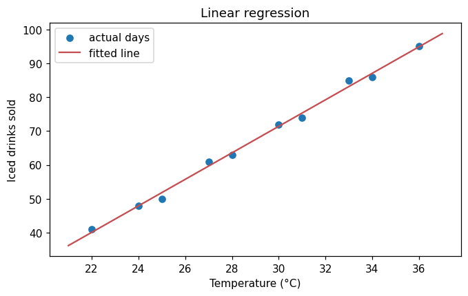

reshape(-1, 1) turns the 1D list of temperatures into a column, because scikit-learn always expects X to be 2D (rows × features). The slope means each extra degree brings about 3.9 more iced drinks, and the line predicts about 67.5 drinks on a 29°C day.

How least squares works#

For one feature the best slope and intercept have a direct formula; computing it by hand gives the same numbers as scikit-learn:

import numpy as np

x = np.array([22, 24, 25, 27, 28, 30, 31, 33, 34, 36])
y = np.array([41, 48, 50, 61, 63, 72, 74, 85, 86, 95])

slope = ((x - x.mean()) * (y - y.mean())).sum() / ((x - x.mean()) ** 2).sum()
intercept = y.mean() - slope * x.mean()
print(round(slope, 2), round(intercept, 2))

3.91 -45.91

With many features the same idea is solved with linear algebra (or iteratively with gradient descent, which you will meet in How Neural Networks Learn).

Residuals#

A residual is the error for one point: actual − predicted. Looking at residuals shows whether a straight line suits the data:

import numpy as np
from sklearn.linear_model import LinearRegression

x = np.array([22, 24, 25, 27, 28, 30, 31, 33, 34, 36]).reshape(-1, 1)
y = np.array([41, 48, 50, 61, 63, 72, 74, 85, 86, 95])
model = LinearRegression().fit(x, y)

residuals = y - model.predict(x)
print(residuals.round(1))
print("mean residual:", round(residuals.mean(), 6))
print("largest miss:", round(np.abs(residuals).max(), 1), "drinks")

[ 0.9  0.1 -1.9  1.3 -0.6  0.6 -1.3  1.9 -1.1  0.1]
mean residual: 0.0
largest miss: 1.9 drinks

Least squares always makes the residuals average to zero. Good residuals look like random noise around 0; a curved pattern (positive at the ends, negative in the middle, for example) means the relationship is not a straight line and a different model is needed (see polynomial regression).

Assumptions and limits#

Linear regression works best when:

• the relationship is roughly linear;
• errors are random, with no pattern over time or across the range;
• there are no extreme outliers (squared errors make outliers very influential).

Also, a line fitted on 22 to 36°C says nothing reliable about 5°C or 45°C: extrapolating far outside the training range is risky.

Common mistakes#

Practice#

import numpy as np
from sklearn.linear_model import LinearRegression

hours = np.array([1, 2, 3, 4, 5, 6, 7, 8]).reshape(-1, 1)
scores = np.array([52, 55, 61, 64, 68, 74, 77, 83])
model = LinearRegression().fit(hours, scores)
print(round(model.coef_[0], 2), round(model.intercept_, 2))
print(round(model.predict([[5.5]])[0], 1))

4.4 46.93
71.2

Key takeaway#

Next: Multiple and Polynomial Regression.