Support Vector Machines (SVM) in Python: Margins and Kernels

A support vector machine (SVM) separates classes with the boundary that leaves the widest possible gap (the margin) between them. The training points closest to the boundary, which determine where it goes, are the support vectors. With kernels, SVMs can also draw curved boundaries. They work well on small and medium datasets with many features.

The maximum-margin idea#

Many lines can separate two well-separated groups. An SVM picks the one furthest from the nearest points of both classes, which tends to generalise best to new points:

import numpy as np
import matplotlib.pyplot as plt
from sklearn.svm import SVC

rng = np.random.default_rng(2)
X = np.vstack([rng.normal([2, 2], 0.6, (25, 2)), rng.normal([5, 5], 0.6, (25, 2))])
y = np.array([0] * 25 + [1] * 25)

model = SVC(kernel="linear", C=1.0).fit(X, y)
print("support vectors:", len(model.support_vectors_))

fig, ax = plt.subplots(figsize=(5.5, 5))
ax.scatter(X[:, 0], X[:, 1], c=y, cmap="coolwarm", s=25)
xx, yy = np.meshgrid(np.linspace(0, 7, 200), np.linspace(0, 7, 200))
zz = model.decision_function(np.c_[xx.ravel(), yy.ravel()]).reshape(xx.shape)
ax.contour(xx, yy, zz, levels=[-1, 0, 1], linestyles=["--", "-", "--"], colors="k")
ax.scatter(model.support_vectors_[:, 0], model.support_vectors_[:, 1], s=120, facecolors="none", edgecolors="k")
ax.set_title("Linear SVM: boundary, margins and support vectors")
plt.show()

support vectors: 2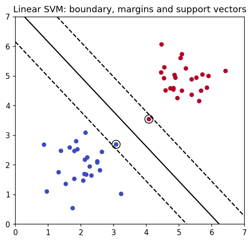

The solid line is the decision boundary, the dashed lines are the margins, and the circled points are the support vectors. Moving any other point (without crossing a margin) would not change the boundary at all.

Soft margins: the C parameter#

Real data overlaps, so a perfect separation is impossible or would overfit. The C parameter controls how much the SVM tolerates points inside the margin or on the wrong side:

• small C: a wider margin that ignores some points (simpler, more regularised);
• large C: a narrower margin that tries hard to classify every training point (risk of overfitting).

Kernels: curved boundaries#

A kernel lets an SVM draw non-linear boundaries by implicitly comparing points in a higher-dimensional space. The RBF (radial basis function) kernel is the default and works well in many problems. Its gamma parameter sets how far each training point's influence reaches: high gamma means very local, wiggly boundaries.

from sklearn.datasets import make_moons
from sklearn.model_selection import train_test_split
from sklearn.svm import SVC

X, y = make_moons(n_samples=300, noise=0.25, random_state=0)
X_train, X_test, y_train, y_test = train_test_split(X, y, test_size=0.3, random_state=0)

for kernel, params in [("linear", {}), ("rbf", {"gamma": 2}), ("rbf", {"gamma": 500})]:
    model = SVC(kernel=kernel, C=1.0, **params).fit(X_train, y_train)
    label = kernel + (f" gamma={params['gamma']}" if params else "")
    print(f"{label:>15}: train {model.score(X_train, y_train):.3f}, test {model.score(X_test, y_test):.3f}")

         linear: train 0.833, test 0.856
    rbf gamma=2: train 0.952, test 0.967
  rbf gamma=500: train 1.000, test 0.700

The two interleaving "moons" cannot be separated by a straight line, so the linear kernel underfits. The RBF kernel with a moderate gamma fits the shape well. With a very high gamma (500), each point's influence is so local that the model memorises the training set: a perfect training score, but a much lower test score.

Scale your features#

SVMs depend on distances, like KNN, so unscaled features distort them. Always use a pipeline with StandardScaler:

from sklearn.datasets import load_wine
from sklearn.model_selection import cross_val_score
from sklearn.pipeline import make_pipeline
from sklearn.preprocessing import StandardScaler
from sklearn.svm import SVC

X, y = load_wine(return_X_y=True)
print("unscaled:", round(cross_val_score(SVC(), X, y, cv=5).mean(), 3))
print("scaled:  ", round(cross_val_score(make_pipeline(StandardScaler(), SVC()), X, y, cv=5).mean(), 3))

unscaled: 0.663
scaled:   0.983

When to use an SVM#

• Good fit: small to medium datasets, many features (including text), clear margins between classes.
• Less suitable: very large datasets (training time grows quickly with the number of rows), problems needing calibrated probabilities (SVMs need extra work, probability=True, to output them), or when you need an easily explained model.

Common mistakes#

Practice#

from sklearn.datasets import make_moons
from sklearn.model_selection import cross_val_score
from sklearn.svm import SVC

X, y = make_moons(n_samples=300, noise=0.25, random_state=0)
for c in [0.1, 1, 100]:
    print(c, round(cross_val_score(SVC(C=c), X, y, cv=5).mean(), 3))

0.1 0.903
1 0.957
100 0.94

Key takeaway#

Next: Feature Engineering.