Machine Learning course menu
Classification Metrics: Confusion Matrix, Precision, Recall, F1 and ROC AUC
Evaluate classifiers properly: why accuracy misleads on imbalanced data, the confusion matrix, precision, recall, F1 score, classification_report, the precision-recall trade-off, ROC curves and AUC, with scikit-learn.
On this page
Accuracy (the share of correct predictions) is the obvious way to score a classifier, and often the wrong one. If 1% of transactions are fraud, a model that always says "not fraud" is 99% accurate and completely useless. Better metrics look at which kinds of mistakes a model makes.
The confusion matrix#
For a yes/no problem, every prediction falls into one of four cells:
import numpy as np
from sklearn.metrics import confusion_matrix

actual    = np.array([0, 0, 0, 0, 0, 0, 1, 1, 1, 1])
predicted = np.array([0, 0, 0, 0, 1, 1, 1, 1, 1, 0])
print(confusion_matrix(actual, predicted))
tn, fp, fn, tp = confusion_matrix(actual, predicted).ravel()
print(f"TN={tn} FP={fp} FN={fn} TP={tp}")[[4 2]
[1 3]]
TN=4 FP=2 FN=1 TP=3scikit-learn puts actual classes in rows and predicted classes in columns, in sorted label order (0 then 1).
Precision, recall and F1#
- Precision = TP / (TP + FP): of everything the model flagged, how much was right? High precision means few false alarms.
- Recall (sensitivity) = TP / (TP + FN): of all real positives, how many did the model catch? High recall means few misses.
- F1 score = the harmonic mean of precision and recall, a single number that is high only when both are.
import numpy as np
from sklearn.metrics import accuracy_score, f1_score, precision_score, recall_score

actual    = np.array([0, 0, 0, 0, 0, 0, 1, 1, 1, 1])
predicted = np.array([0, 0, 0, 0, 1, 1, 1, 1, 1, 0])
print("accuracy ", accuracy_score(actual, predicted))
print("precision", precision_score(actual, predicted))
print("recall   ", recall_score(actual, predicted))
print("F1 ", round(f1_score(actual, predicted), 3))accuracy 0.7
precision 0.6
recall 0.75
F1 0.667With 3 true positives, 2 false alarms and 1 miss: precision is 3/5 = 0.6 and recall is 3/4 = 0.75.
Which matters more?#
The accuracy paradox#
import numpy as np
from sklearn.metrics import accuracy_score, recall_score

actual = np.array([0] * 990 + [1] * 10)          # 1% positives
lazy = np.zeros(1000, dtype=int)                  # always predict negative
print("accuracy:", accuracy_score(actual, lazy))
print("recall: ", recall_score(actual, lazy))accuracy: 0.99
recall: 0.099% accurate, 0% of positives found. On imbalanced data, report precision, recall and F1 (see Imbalanced Data).
classification_report#
One call prints the per-class metrics for a real model:
from sklearn.datasets import load_breast_cancer
from sklearn.linear_model import LogisticRegression
from sklearn.metrics import classification_report, confusion_matrix
from sklearn.model_selection import train_test_split
from sklearn.pipeline import make_pipeline
from sklearn.preprocessing import StandardScaler

X, y = load_breast_cancer(return_X_y=True)
X_train, X_test, y_train, y_test = train_test_split(X, y, test_size=0.25, random_state=0, stratify=y)
model = make_pipeline(StandardScaler(), LogisticRegression()).fit(X_train, y_train)
predicted = model.predict(X_test)
print(confusion_matrix(y_test, predicted))
print(classification_report(y_test, predicted, target_names=["malignant", "benign"]))[[50 3]
[ 3 87]]
precision recall f1-score support
malignant 0.94 0.94 0.94 53
benign 0.97 0.97 0.97 90
accuracy 0.96 143
macro avg 0.96 0.96 0.96 143
weighted avg 0.96 0.96 0.96 143The support column is the number of real examples of each class. The macro average weights both classes equally; the weighted average weights them by support.
The precision-recall trade-off and ROC AUC#
Changing the decision threshold trades precision against recall. The ROC curve plots the true positive rate (recall) against the false positive rate for every threshold, and the AUC (area under it) summarises how well the model ranks positives above negatives: 0.5 is random guessing, 1.0 is perfect.
import matplotlib.pyplot as plt
from sklearn.datasets import load_breast_cancer
from sklearn.linear_model import LogisticRegression
from sklearn.metrics import RocCurveDisplay, roc_auc_score
from sklearn.model_selection import train_test_split
from sklearn.pipeline import make_pipeline
from sklearn.preprocessing import StandardScaler
from sklearn.tree import DecisionTreeClassifier

X, y = load_breast_cancer(return_X_y=True)
X_train, X_test, y_train, y_test = train_test_split(X, y, test_size=0.25, random_state=0, stratify=y)
logistic = make_pipeline(StandardScaler(), LogisticRegression()).fit(X_train, y_train)
stump = DecisionTreeClassifier(max_depth=1, random_state=0).fit(X_train, y_train)

fig, ax = plt.subplots(figsize=(5.5, 5))
RocCurveDisplay.from_estimator(logistic, X_test, y_test, name="logistic regression", ax=ax)
RocCurveDisplay.from_estimator(stump, X_test, y_test, name="one-split tree", ax=ax)
ax.plot([0, 1], [0, 1], linestyle="--", color="grey", label="random guess")
ax.legend()
plt.show()
for name, m in [("logistic", logistic), ("stump", stump)]:
print(name, round(roc_auc_score(y_test, m.predict_proba(X_test)[:, 1]), 3))logistic 0.995
stump 0.884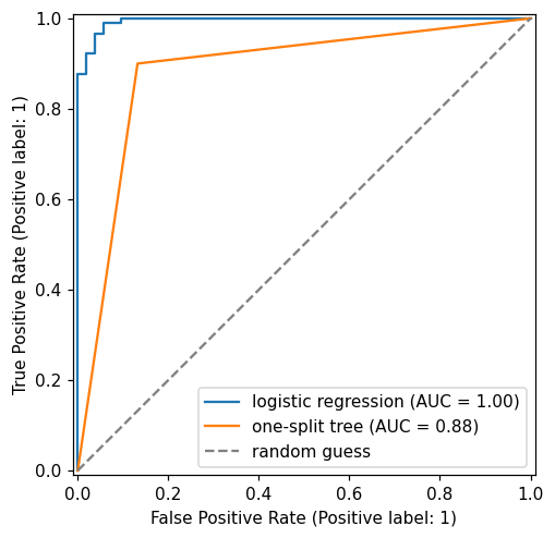
The curve closer to the top-left corner is better. AUC needs probabilities (predict_proba), not hard predictions, and it does not depend on any particular threshold.
Common mistakes#
Practice#
Practice exercise
A screening model's predictions for 12 patients are actual = [1, 0, 1, 1, 0, 0, 1, 0, 0, 1, 0, 0] and predicted = [1, 0, 0, 1, 0, 1, 1, 0, 0, 1, 0, 0]. Print the confusion matrix, precision, recall and F1 (3 decimals). For a cancer screening test, which number worries you most?
Show hint
Use confusion_matrix, precision_score, recall_score and f1_score from sklearn.metrics.
Show solution
from sklearn.metrics import confusion_matrix, f1_score, precision_score, recall_score

actual    = [1, 0, 1, 1, 0, 0, 1, 0, 0, 1, 0, 0]
predicted = [1, 0, 0, 1, 0, 1, 1, 0, 0, 1, 0, 0]
print(confusion_matrix(actual, predicted))
print(round(precision_score(actual, predicted), 3), round(recall_score(actual, predicted), 3), round(f1_score(actual, predicted), 3))[[6 1]
[1 4]]
0.8 0.8 0.8The recall of 0.8 means one patient with cancer in five was missed (one false negative). For screening, that miss matters far more than the single false alarm.
Key takeaway#
Next: k-Nearest Neighbours.
Finished this lesson?