Machine Learning course menu
Anomaly Detection in Python: Isolation Forest and More
Find unusual data points without labels: statistical rules, Isolation Forest, Local Outlier Factor, setting the contamination rate, anomaly scores, and evaluating detectors when a few labelled cases exist.
On this page
Anomaly detection finds rare, unusual cases: a fraudulent transaction, a failing machine, a hacked account, a sensor gone wrong. Often there are few or no labelled examples of anomalies (they are rare and keep changing), so the methods learn what normal looks like and flag what does not fit.
Simple statistical rules first#
For a single numeric value, the IQR rule or z-scores are often enough. Machine learning methods help when anomalies are unusual combinations of features: a ₹2,000 purchase is normal, and a purchase at 3 a.m. is normal, but a ₹2,000 purchase at 3 a.m. from a new device may not be.
Isolation Forest#
An Isolation Forest builds random trees that split the data at random thresholds. Unusual points are easy to separate from the rest, so they end up isolated after only a few splits; normal points sit in dense regions and take many splits. Points with short average paths get high anomaly scores.
import numpy as np
import matplotlib.pyplot as plt
from sklearn.ensemble import IsolationForest

rng = np.random.default_rng(1)
normal = rng.normal([50, 30], [8, 5], size=(300, 2))           # amount (₹ hundreds), hour-ish feature
odd = np.array([[95, 5], [10, 55], [90, 52], [5, 2], [98, 30]])
X = np.vstack([normal, odd])

detector = IsolationForest(contamination=0.02, random_state=0).fit(X)
flags = detector.predict(X)                       # -1 = anomaly, 1 = normal
print("flagged:", int((flags == -1).sum()), "of", len(X))
print("the 5 planted points flagged:", int((flags[-5:] == -1).sum()))

fig, ax = plt.subplots(figsize=(6, 4.5))
ax.scatter(X[flags == 1, 0], X[flags == 1, 1], s=12, label="normal")
ax.scatter(X[flags == -1, 0], X[flags == -1, 1], s=60, marker="x", color="#C44E52", label="flagged")
ax.set(xlabel="feature 1", ylabel="feature 2", title="Isolation Forest")
ax.legend()
plt.show()flagged: 7 of 305
the 5 planted points flagged: 5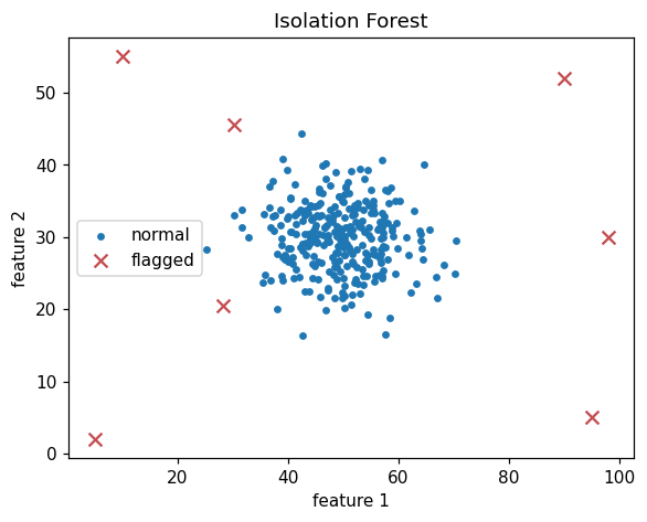
contamination tells the model what share of points to flag. Here it is set to 2%, so the model flags roughly 2% of the 305 points (7 in this run): all five planted anomalies, plus two of the most extreme normal points.
Anomaly scores#
Instead of a hard yes/no, use the score to rank cases for investigation, so a team can review the most suspicious first:
import numpy as np
from sklearn.ensemble import IsolationForest

rng = np.random.default_rng(1)
normal = rng.normal([50, 30], [8, 5], size=(300, 2))
odd = np.array([[95, 5], [10, 55], [90, 52], [5, 2], [98, 30]])
X = np.vstack([normal, odd])
detector = IsolationForest(random_state=0).fit(X)

scores = -detector.score_samples(X)               # higher = more anomalous
top = np.argsort(scores)[::-1][:5]
print("most anomalous rows:", top.tolist())
print("their scores:", scores[top].round(3).tolist())most anomalous rows: [303, 301, 300, 302, 304]
their scores: [0.82, 0.798, 0.795, 0.792, 0.731]The five planted points (rows 300–304) take the top five places.
Local Outlier Factor#
Local Outlier Factor (LOF) compares each point's local density with its neighbours' density. It finds points that are unusual relative to their own neighbourhood, which helps when normal data has clusters of different densities:
import numpy as np
from sklearn.neighbors import LocalOutlierFactor

rng = np.random.default_rng(2)
dense = rng.normal(0, 0.3, size=(100, 2))
sparse = rng.normal(5, 1.5, size=(100, 2))
odd = np.array([[1.5, 1.5]])                      # far from the dense cluster, but within normal spread overall
X = np.vstack([dense, sparse, odd])

lof = LocalOutlierFactor(n_neighbors=20, contamination=0.01)
labels = lof.fit_predict(X)
print("is the odd point flagged?", labels[-1] == -1)
print("flagged count:", int((labels == -1).sum()))is the odd point flagged? True
flagged count: 2The point at (1.5, 1.5) would look ordinary next to the sparse cluster, but it is far outside the dense cluster it sits beside, so LOF flags it.
Evaluating with a few labels#
If you have even a handful of confirmed anomalies, use them to evaluate and choose settings, ranking by score and measuring precision among the top flagged cases:
import numpy as np
from sklearn.ensemble import IsolationForest
from sklearn.metrics import average_precision_score

rng = np.random.default_rng(1)
normal = rng.normal([50, 30], [8, 5], size=(300, 2))
odd = np.array([[95, 5], [10, 55], [90, 52], [5, 2], [98, 30]])
X = np.vstack([normal, odd])
is_anomaly = np.r_[np.zeros(300), np.ones(5)]

scores = -IsolationForest(random_state=0).fit(X).score_samples(X)
print("average precision:", round(average_precision_score(is_anomaly, scores), 3))
top10 = np.argsort(scores)[::-1][:10]
print("anomalies among the top 10:", int(is_anomaly[top10].sum()))average precision: 1.0
anomalies among the top 10: 5Once enough labelled examples accumulate, a supervised classifier (with the techniques from Imbalanced Data) usually outperforms unsupervised detection; many systems combine both.
Common mistakes#
Practice#
Practice exercise
Daily server response times (ms) are normally around 120 ± 15, with a few incidents. Simulate 500 normal days plus incidents [400, 380, 30, 410], fit an IsolationForest(random_state=0) on the single feature, and print the 4 most anomalous values.
Show hint
Reshape to a column with reshape(-1, 1); sort by -score_samples(X) and take the top 4 rows.
Show solution
import numpy as np
from sklearn.ensemble import IsolationForest

rng = np.random.default_rng(4)
times = np.r_[rng.normal(120, 15, 500), [400, 380, 30, 410]].reshape(-1, 1)
scores = -IsolationForest(random_state=0).fit(times).score_samples(times)
top4 = np.argsort(scores)[::-1][:4]
print(np.sort(times[top4].ravel()).round(0))[ 30. 380. 400. 410.]For a single feature like this, a simple percentile rule would find the same days; Isolation Forest earns its place when anomalies are combinations of several features.
Key takeaway#
Next, neural networks: How Neural Networks Learn.
Finished this lesson?