Machine Learning course menu
Machine Learning Project: House Price Prediction in Python
A complete regression project from start to finish: exploring housing data, a baseline, preprocessing numeric and categorical features in a pipeline, comparing linear regression and gradient boosting with cross-validation, analysing errors, feature importance, and saving the final model.
On this page
This project walks through a full regression workflow: predicting flat prices from size, location and other features. Each step builds on the previous one, so run them in order.
Goal: predict the sale price of a flat (in lakh rupees) so an estate agency can suggest a fair asking price. The agency wants the typical error well under 10% of the price.
Step 1: The data#
The data is simulated so the lesson runs anywhere without downloads, but it is built to behave like real listings: price depends on area, location, age, floor and amenities, with noise.
import numpy as np
import pandas as pd

rng = np.random.default_rng(42)
n = 1500
area_type = rng.choice(["central", "suburb", "outskirts"], size=n, p=[0.25, 0.5, 0.25])
sqft = rng.normal(1100, 300, n).clip(400, 2600).round()
bedrooms = np.clip(np.round(sqft / 450 + rng.normal(0, 0.5, n)), 1, 5).astype(int)
age = rng.integers(0, 30, n)
floor = rng.integers(0, 15, n)
parking = rng.random(n) < 0.6

rate = pd.Series(area_type).map({"central": 9.0, "suburb": 6.0, "outskirts": 4.0}).to_numpy()   # thousand ₹ per sq ft
price = sqft * rate / 100 * (1 - 0.008 * age) * (1 + 0.01 * np.minimum(floor, 10)) + 6 * parking
price = price * rng.normal(1, 0.08, n)                         # unexplained variation

flats = pd.DataFrame({"sqft": sqft, "bedrooms": bedrooms, "age": age, "floor": floor,
                      "parking": parking, "area_type": area_type, "price_lakh": price.round(1)})
print(flats.shape)
print(flats.head())(1500, 7)
sqft bedrooms age floor parking area_type price_lakh
0 1389.0 2 16 2 False outskirts 49.1
1 883.0 2 19 5 True suburb 49.8
2 844.0 2 29 8 True outskirts 34.2
3 1238.0 2 22 0 True suburb 64.9
4 1397.0 3 6 1 True central 138.0Step 2: Explore#
print(flats.describe().round(1).loc[["mean", "min", "max"]])
print(flats.groupby("area_type")["price_lakh"].median().sort_values())
print("correlation with price:")
print(flats[["sqft", "bedrooms", "age", "floor"]].corrwith(flats["price_lakh"]).round(2)) sqft bedrooms age floor price_lakh
mean 1088.4 2.4 14.6 7.0 67.7
min 400.0 1.0 0.0 0.0 12.1
max 2018.0 5.0 29.0 14.0 198.4
area_type
outskirts 44.5
suburb 64.2
central 96.1
Name: price_lakh, dtype: float64
correlation with price:
sqft 0.64
bedrooms 0.50
age -0.20
floor 0.05
dtype: float64Size matters most, and location shifts prices strongly: a typical central flat costs more than twice as much as one on the outskirts. Bedrooms correlate with price mainly because they go with size. Age has a weak negative correlation on its own.
Step 3: Split and baseline#
Hold back a test set before any modelling, and compute a baseline: predicting the median training price for every flat.
from sklearn.metrics import mean_absolute_error
from sklearn.model_selection import train_test_split

X = flats.drop(columns="price_lakh")
y = flats["price_lakh"]
X_train, X_test, y_train, y_test = train_test_split(X, y, test_size=0.2, random_state=0)

baseline = mean_absolute_error(y_test, np.full(len(y_test), y_train.median()))
print(f"baseline MAE: {baseline:.1f} lakh (typical price {y_train.median():.1f} lakh)")baseline MAE: 22.0 lakh (typical price 64.3 lakh)Any useful model must beat this by a wide margin.
Step 4: Preprocessing and models#
area_type is text, so it needs one-hot encoding; numeric columns are scaled for the linear model. A ColumnTransformer inside a pipeline handles both, and cross-validation compares models fairly on the training data only:
from sklearn.compose import ColumnTransformer
from sklearn.ensemble import HistGradientBoostingRegressor
from sklearn.linear_model import LinearRegression
from sklearn.model_selection import cross_val_score
from sklearn.pipeline import make_pipeline
from sklearn.preprocessing import OneHotEncoder, StandardScaler

numeric = ["sqft", "bedrooms", "age", "floor", "parking"]
categorical = ["area_type"]
preprocess = ColumnTransformer([
    ("num", StandardScaler(), numeric),
    ("cat", OneHotEncoder(handle_unknown="ignore"), categorical),
])

models = {
    "linear regression": make_pipeline(preprocess, LinearRegression()),
    "gradient boosting": make_pipeline(preprocess, HistGradientBoostingRegressor(random_state=0)),
}
for name, model in models.items():
    mae = -cross_val_score(model, X_train, y_train, cv=5, scoring="neg_mean_absolute_error").mean()
print(f"{name}: cross-validated MAE {mae:.2f} lakh")linear regression: cross-validated MAE 5.95 lakh
gradient boosting: cross-validated MAE 5.09 lakhBoth beat the baseline easily. Gradient boosting does better than plain linear regression: price depends on size times a location rate, an interaction that a straight-line model cannot express with these features but trees learn naturally.
Step 5: Improve the linear model with a feature#
Domain knowledge can close the gap: give the linear model the interaction directly, as size per location.
from sklearn.preprocessing import FunctionTransformer

def add_location_size(df):
    df = df.copy()
    for area in ["central", "suburb", "outskirts"]:
        df[f"sqft_{area}"] = df["sqft"] * (df["area_type"] == area)
    return df

numeric_plus = numeric + ["sqft_central", "sqft_suburb", "sqft_outskirts"]
preprocess_plus = ColumnTransformer([
    ("num", StandardScaler(), numeric_plus),
    ("cat", OneHotEncoder(handle_unknown="ignore"), categorical),
])
linear_plus = make_pipeline(FunctionTransformer(add_location_size), preprocess_plus, LinearRegression())
mae = -cross_val_score(linear_plus, X_train, y_train, cv=5, scoring="neg_mean_absolute_error").mean()
print(f"linear regression + size-by-location features: cross-validated MAE {mae:.2f} lakh")linear regression + size-by-location features: cross-validated MAE 4.72 lakhOne well-chosen feature made the simple linear model the best of the three, ahead of gradient boosting, while staying easy to explain. This is the value of feature engineering.
Step 6: Final evaluation on the test set#
Cross-validation picked the linear model with size-by-location features. Evaluate it once on the untouched test set:
from sklearn.metrics import r2_score

final = linear_plus.fit(X_train, y_train)
pred = final.predict(X_test)
mae = mean_absolute_error(y_test, pred)
pct = (np.abs(pred - y_test) / y_test).median()
print(f"test MAE: {mae:.2f} lakh, R²: {r2_score(y_test, pred):.3f}")
print(f"median error: {pct:.1%} of the price")test MAE: 4.68 lakh, R²: 0.952
median error: 6.2% of the priceThe goal was a typical error well under 10% of the price, so the model meets it. Part of the remaining error is the random 8% variation built into the data, which no model can predict: real prices also depend on things the data does not record.
Step 7: Check the errors#
import matplotlib.pyplot as plt

fig, ax = plt.subplots(figsize=(6, 4.5))
ax.scatter(y_test, pred, s=10, alpha=0.6)
lims = [y_test.min(), y_test.max()]
ax.plot(lims, lims, color="#C44E52", label="perfect prediction")
ax.set(xlabel="actual price (lakh ₹)", ylabel="predicted price (lakh ₹)", title="Predicted vs actual on the test set")
ax.legend()
plt.show()

errors = pd.DataFrame({"area_type": X_test["area_type"], "abs_error": np.abs(pred - y_test)})
print(errors.groupby("area_type")["abs_error"].mean().round(2))area_type
central 6.44
outskirts 3.61
suburb 4.25
Name: abs_error, dtype: float64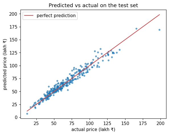
Errors in rupees are largest for central flats simply because they cost more; the percentage error is similar across areas. If errors were much worse for one area, that would point to too little data or a missing feature there.
Step 8: What drives predictions?#
Permutation importance shuffles one feature at a time on the test set and measures how much the error grows:
from sklearn.inspection import permutation_importance

result = permutation_importance(final, X_test, y_test, scoring="neg_mean_absolute_error",
                                n_repeats=5, random_state=0)
importance = pd.Series(result.importances_mean, index=X_test.columns).sort_values(ascending=False)
print(importance.round(2))area_type 16.77
sqft 15.67
age 2.63
parking 1.01
floor 0.40
bedrooms 0.05
dtype: float64Size and location dominate, followed by age, parking and floor. Bedrooms add almost nothing once size is known, which matches how the data was generated, a useful sanity check.
Step 9: Save the model#
import joblib

final_model = linear_plus.fit(X, y)          # refit on all the data
joblib.dump(final_model, "house_price_model.joblib")
example = pd.DataFrame([{"sqft": 1200, "bedrooms": 3, "age": 5, "floor": 4, "parking": True, "area_type": "suburb"}])
print(f"suggested price: {joblib.load('house_price_model.joblib').predict(example)[0]:.1f} lakh")suggested price: 78.2 lakhThe pipeline contains our own function, add_location_size. Pickle files store a reference to such a function, not its code, so any program that loads the model must be able to import it. In a real project, put helper functions like this in a module (for example features.py) that both the training script and the API import.
After choosing and testing the approach, refitting on all the data gives the final model the most information. It can now be served through an API.
What you practised#
- exploring data and setting a baseline before modelling;
- a
ColumnTransformerpipeline for mixed numeric and categorical features; - comparing models with cross-validation, and feature engineering to improve a simple model;
- one final test-set evaluation, error analysis and permutation importance;
- saving the final model.
Practice exercise
Extend the project: add a price_per_sqft column to the explore step and print its median for each area_type. Why must you not use price_per_sqft as a model feature?
Show hint
Divide price_lakh * 100000 by sqft. Think about what you would need to know to compute it for a new flat.
Show solution
per_sqft = flats["price_lakh"] * 100000 / flats["sqft"]
print(per_sqft.groupby(flats["area_type"]).median().round(0))area_type
central 8730.0
outskirts 4115.0
suburb 5962.0
dtype: float64price_per_sqft is computed from the price itself, which is exactly what the model is supposed to predict. For a new flat it is unknown, and using it in training would be target leakage: excellent scores in testing, useless in practice.
Next project: Customer Churn Prediction.
Finished this lesson?