Machine Learning course menu

Multiple and Polynomial Regression in scikit-learn

Extend linear regression to many features, interpret coefficients, compare features on a common scale with standardisation, model curved relationships with PolynomialFeatures, and see how too high a degree overfits.

Beginner9 min readUpdated October 24, 2026

On this page

Several features
Comparing feature importance
Polynomial regression: curves
Common mistakes
Practice
Key takeaway

Real predictions depend on many things at once: a house price depends on its area, bedrooms, age and location. Multiple regression uses several features; polynomial regression bends the line to follow curves. Both are still "linear" models underneath, and both use LinearRegression.

Several features#

With features x₁, x₂, …, the model adds one coefficient per feature:

Text

prediction = intercept + w₁·x₁ + w₂·x₂ + … + wₙ·xₙ

We will use simulated house data where the true effects are known, so you can see the model recover them:

Python

import numpy as np
import pandas as pd
from sklearn.linear_model import LinearRegression
from sklearn.model_selection import train_test_split

rng = np.random.default_rng(0)
n = 300
houses = pd.DataFrame({
    "area_sqft": rng.integers(500, 2500, n),
    "bedrooms": rng.integers(1, 5, n),
    "age_years": rng.integers(0, 40, n),
})
houses["price_lakh"] = (10 + 0.06 * houses["area_sqft"] + 4 * houses["bedrooms"]
                        - 0.5 * houses["age_years"] + rng.normal(0, 8, n)).round(1)

X = houses.drop(columns="price_lakh")
y = houses["price_lakh"]
X_train, X_test, y_train, y_test = train_test_split(X, y, test_size=0.25, random_state=0)

model = LinearRegression().fit(X_train, y_train)
print(pd.Series(model.coef_, index=X.columns).round(3))
print("intercept:", round(model.intercept_, 2))
print("test R²:", round(model.score(X_test, y_test), 3))

Output

area_sqft    0.059
bedrooms     3.948
age_years   -0.541
dtype: float64
intercept: 12.41
test R²: 0.959

The model recovered values close to the true ones (0.06 per square foot, 4 per bedroom, −0.5 per year of age). Each coefficient means: holding the other features fixed, one more unit of this feature changes the predicted price by this much.

Comparing feature importance#

Raw coefficients depend on units: 0.06 per square foot is not "smaller" than 4 per bedroom, because areas are in the thousands. Standardising the features (mean 0, standard deviation 1) puts every coefficient on the same scale, "change per standard deviation":

Python

import numpy as np
import pandas as pd
from sklearn.linear_model import LinearRegression
from sklearn.preprocessing import StandardScaler

rng = np.random.default_rng(0)
n = 300
X = pd.DataFrame({
    "area_sqft": rng.integers(500, 2500, n),
    "bedrooms": rng.integers(1, 5, n),
    "age_years": rng.integers(0, 40, n),
})
y = 10 + 0.06 * X["area_sqft"] + 4 * X["bedrooms"] - 0.5 * X["age_years"] + rng.normal(0, 8, n)

X_scaled = StandardScaler().fit_transform(X)
model = LinearRegression().fit(X_scaled, y)
print(pd.Series(model.coef_, index=X.columns).round(2).sort_values(key=abs, ascending=False))

Output

area_sqft    35.41
age_years    -5.75
bedrooms      4.84
dtype: float64

Area has by far the biggest effect per standard deviation. (Strongly correlated features make coefficients unstable and hard to interpret; regularisation, next lesson, helps.)

Polynomial regression: curves#

When the relationship curves, add powers of the feature (x², x³, …) as new columns, then fit an ordinary linear regression on them. PolynomialFeatures creates the columns:

Python

import numpy as np
from sklearn.preprocessing import PolynomialFeatures

x = np.array([[2], [3], [4]])
print(PolynomialFeatures(degree=3, include_bias=False).fit_transform(x))

Output

[[ 2.  4.  8.]
 [ 3.  9. 27.]
 [ 4. 16. 64.]]

Comparing degrees on curved data shows both underfitting and overfitting:

Python

import numpy as np
import matplotlib.pyplot as plt
from sklearn.linear_model import LinearRegression
from sklearn.model_selection import train_test_split
from sklearn.pipeline import make_pipeline
from sklearn.preprocessing import PolynomialFeatures

rng = np.random.default_rng(3)
x = np.sort(rng.uniform(0, 6, 40)).reshape(-1, 1)
y = np.sin(x).ravel() * 10 + rng.normal(0, 1.5, 40)
x_train, x_test, y_train, y_test = train_test_split(x, y, test_size=0.3, random_state=1)

fig, axes = plt.subplots(1, 3, figsize=(13, 3.8), sharey=True)
grid = np.linspace(0, 6, 200).reshape(-1, 1)
for ax, degree in zip(axes, [1, 4, 15]):
    model = make_pipeline(PolynomialFeatures(degree, include_bias=False), LinearRegression())
    model.fit(x_train, y_train)
    ax.scatter(x_train, y_train, s=15, label="train")
    ax.scatter(x_test, y_test, s=15, marker="x", label="test")
    ax.plot(grid, model.predict(grid), color="#C44E52")
    ax.set_ylim(-20, 20)
    ax.set_title(f"degree {degree}: train R² {model.score(x_train, y_train):.2f}, test R² {model.score(x_test, y_test):.2f}")
    print(degree, round(model.score(x_train, y_train), 3), round(model.score(x_test, y_test), 3))
axes[0].legend()
fig.tight_layout()
plt.show()

Output

1 0.58 0.502
4 0.964 0.939
15 0.977 0.927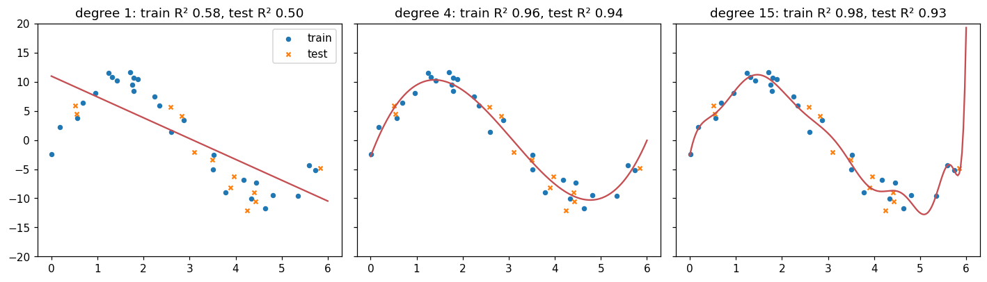

Three panels fitting the same wavy data: a straight line that misses the curve, a smooth degree-4 curve that follows it well, and a degree-15 curve that wiggles to pass near the training points but swings wildly elsewhere.

Degree 1 (a straight line) underfits: it cannot follow the curve, so both scores are low.
Degree 4 captures the shape and scores well on both training and test data.
Degree 15 overfits: it bends to chase noise in the training points, so its training score is the highest but its test score drops.

The test score, not the training score, decides which model is best. Cross-validation picks the degree systematically.

Common mistakes#

Practice#

Practice exercise

Using load_diabetes(return_X_y=True, as_frame=True), split 80/20 with random_state=0, fit a linear regression on all features, and print the test R² (3 decimals) and the three features with the largest absolute coefficients. (The features in this dataset are already scaled.)

Show hint

as_frame=True returns a DataFrame, so you can label the coefficients with X.columns, then sort by absolute value with sort_values(key=abs).

Show solution

Python

import pandas as pd
from sklearn.datasets import load_diabetes
from sklearn.linear_model import LinearRegression
from sklearn.model_selection import train_test_split

X, y = load_diabetes(return_X_y=True, as_frame=True)
X_train, X_test, y_train, y_test = train_test_split(X, y, test_size=0.2, random_state=0)
model = LinearRegression().fit(X_train, y_train)
print(round(model.score(X_test, y_test), 3))
coefs = pd.Series(model.coef_, index=X.columns)
print(coefs.sort_values(key=abs, ascending=False).head(3).round(1))

Output

0.332
s5     731.6
s1    -662.7
bmi    562.8
dtype: float64

Key takeaway#

Next: Regularisation: Ridge and Lasso.

Finished this lesson?

Machine LearningLinear Regression in Python with scikit-learn (Explained Simply)Learn linear regression: fitting a straight line to data, the slope and intercept, how least squares works, training LinearRegression in scikit-learn, interpreting coefficients, making predictions and checking residuals.Beginner6 min read Machine LearningRidge and Lasso Regression: Regularisation ExplainedLearn regularisation for linear models: why large coefficients overfit, Ridge (L2) and Lasso (L1) penalties, the alpha parameter, how Lasso selects features by setting coefficients to zero, ElasticNet, and why scaling matters.Intermediate7 min read Machine LearningOverfitting, Underfitting and the Bias-Variance Trade-offUnderstand overfitting and underfitting, bias and variance, how to diagnose them with training vs validation scores, validation curves and learning curves in scikit-learn, and the practical fixes for each.Intermediate8 min read

Several features#

Comparing feature importance#

Polynomial regression: curves#

Common mistakes#

Practice#

Key takeaway#

Related lessons