Machine Learning course menu
Principal Component Analysis (PCA) in Python Explained
Learn PCA for dimensionality reduction: finding the directions of greatest variance, explained variance ratio, choosing the number of components, visualising high-dimensional data in 2D, speeding up models, and the limits of PCA.
On this page
Datasets often have many features, and many of them overlap: height in centimetres and height in inches, or ten measurements that all reflect "tumour size". Principal component analysis (PCA) finds a small number of new features, principal components, that capture most of the information (variance) in the original ones.
Uses of PCA:
- Visualise high-dimensional data in two or three dimensions.
- Compress data and speed up models with many features.
- Remove redundancy between correlated features.
The idea#
PCA finds the direction in which the data varies most (the first principal component), then the next direction at right angles to it that captures the most remaining variance, and so on. Each component is a weighted combination of the original features.
import numpy as np
from sklearn.decomposition import PCA

rng = np.random.default_rng(0)
x = rng.normal(0, 1, 200)
data = np.column_stack([x, 2 * x + rng.normal(0, 0.3, 200)])   # two strongly related features

pca = PCA().fit(data)
print("explained variance ratio:", pca.explained_variance_ratio_.round(3))
print("first component direction:", pca.components_[0].round(3))explained variance ratio: [0.996 0.004]
first component direction: [0.444 0.896]Almost all the variation lies along one direction, so one component keeps nearly all the information that two features held.
Seeing 30 dimensions in 2#
The breast cancer data has 30 features. Projected onto its first two principal components, the two diagnoses separate clearly:
import matplotlib.pyplot as plt
from sklearn.datasets import load_breast_cancer
from sklearn.decomposition import PCA
from sklearn.preprocessing import StandardScaler

data = load_breast_cancer()
X = StandardScaler().fit_transform(data.data)
pca = PCA(n_components=2)
X2 = pca.fit_transform(X)
print("variance kept by 2 components:", round(pca.explained_variance_ratio_.sum(), 3))

fig, ax = plt.subplots(figsize=(6.5, 4.5))
for label, name in enumerate(data.target_names):
    ax.scatter(X2[data.target == label, 0], X2[data.target == label, 1], s=12, alpha=0.7, label=name)
ax.set(xlabel="principal component 1", ylabel="principal component 2", title="Breast cancer data in two dimensions")
ax.legend()
plt.show()variance kept by 2 components: 0.632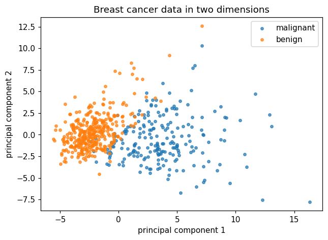
PCA did not use the labels at all, yet the classes separate; that tells you the features carry strong signal. Scale first: PCA looks for variance, so unscaled features with large numbers would dominate.
How many components?#
Plot or print the cumulative explained variance and keep enough components to reach a target such as 90% or 95%:
import numpy as np
from sklearn.datasets import load_breast_cancer
from sklearn.decomposition import PCA
from sklearn.preprocessing import StandardScaler

X = StandardScaler().fit_transform(load_breast_cancer().data)
cumulative = np.cumsum(PCA().fit(X).explained_variance_ratio_)
for k in [1, 2, 5, 7, 10]:
    print(f"{k:>2} components keep {cumulative[k - 1]:.1%} of the variance")
print("components for 95%:", int(np.argmax(cumulative >= 0.95)) + 1)
print("same with PCA(0.95):", PCA(n_components=0.95).fit(X).n_components_) 1 components keep 44.3% of the variance
2 components keep 63.2% of the variance
5 components keep 84.7% of the variance
7 components keep 91.0% of the variance
10 components keep 95.2% of the variance
components for 95%: 10
same with PCA(0.95): 10Passing a fraction such as PCA(n_components=0.95) keeps just enough components to reach that share of the variance.
PCA before a model#
from sklearn.datasets import load_digits
from sklearn.decomposition import PCA
from sklearn.linear_model import LogisticRegression
from sklearn.model_selection import cross_val_score
from sklearn.pipeline import make_pipeline
from sklearn.preprocessing import StandardScaler

X, y = load_digits(return_X_y=True)                 # 8x8 images: 64 features
print("features:", X.shape[1])
for n in [10, 20, 40]:
    model = make_pipeline(StandardScaler(), PCA(n_components=n), LogisticRegression(max_iter=2000))
    print(f"{n} components: accuracy {cross_val_score(model, X, y, cv=5).mean():.3f}")
full = make_pipeline(StandardScaler(), LogisticRegression(max_iter=2000))
print(f"all 64 features: accuracy {cross_val_score(full, X, y, cv=5).mean():.3f}")features: 64
10 components: accuracy 0.840
20 components: accuracy 0.899
40 components: accuracy 0.914
all 64 features: accuracy 0.920Twenty components (under a third of the features) reach 0.899 against 0.920 with all 64, and 40 components close most of the remaining gap. On large datasets that saving matters for speed and memory. Fit PCA inside the pipeline, so it learns only from training folds.
Limits#
- Components are mixtures of all features, which makes them hard to explain ("component 1 is 0.22 × radius + 0.21 × perimeter + …").
- PCA finds linear structure. Curved structure needs non-linear methods such as t-SNE or UMAP (for visualisation).
- High variance is not always what matters for prediction; occasionally a low-variance direction carries the signal.
Common mistakes#
Practice#
Practice exercise
On the wine dataset (13 features), scale the features and print how many principal components are needed to keep 80%, 90% and 95% of the variance.
Show hint
PCA(n_components=fraction).fit(X_scaled).n_components_ for each fraction.
Show solution
from sklearn.datasets import load_wine
from sklearn.decomposition import PCA
from sklearn.preprocessing import StandardScaler

X = StandardScaler().fit_transform(load_wine().data)
for target in [0.8, 0.9, 0.95]:
print(target, PCA(n_components=target).fit(X).n_components_)0.8 5
0.9 8
0.95 10Key takeaway#
Next: Anomaly Detection.
Finished this lesson?