k-Means Clustering in Python: Customer Segmentation Example

Clustering groups similar items together without any labels. It is the most common kind of unsupervised learning: segmenting customers by behaviour, grouping documents by topic, or finding similar products. k-means is the classic clustering algorithm.

How k-means works#

You choose the number of clusters, k. Then:

1. Place k centroids (cluster centres), for example at random points.
2. Assign each point to its nearest centroid.
3. Move each centroid to the average of the points assigned to it.
4. Repeat steps 2 and 3 until the assignments stop changing.

import numpy as np

points = np.array([[1, 1], [1.5, 2], [1, 1.5], [8, 8], [8.5, 9], [9, 8]])
centroids = np.array([[1, 1], [1.5, 2]])           # a poor start: both in one group
for step in range(1, 4):
    distances = np.linalg.norm(points[:, None] - centroids[None], axis=2)
    labels = distances.argmin(axis=1)
    centroids = np.array([points[labels == k].mean(axis=0) for k in range(2)])
    print(f"step {step}: labels {labels.tolist()}, centroids {centroids.round(2).tolist()}")

step 1: labels [0, 1, 0, 1, 1, 1], centroids [[1.0, 1.25], [6.75, 6.75]]
step 2: labels [0, 0, 0, 1, 1, 1], centroids [[1.17, 1.5], [8.5, 8.33]]
step 3: labels [0, 0, 0, 1, 1, 1], centroids [[1.17, 1.5], [8.5, 8.33]]

Even from a poor start, the centroids move to the two natural groups within a couple of steps. scikit-learn's KMeans uses a smarter starting method (k-means++) and runs several starts, keeping the best.

Segmenting customers#

Simulated customers described by annual spend and number of orders:

import numpy as np
import pandas as pd
import matplotlib.pyplot as plt
from sklearn.cluster import KMeans
from sklearn.preprocessing import StandardScaler

rng = np.random.default_rng(3)
groups = [((8000, 4), 120), ((30000, 25), 60), ((15000, 10), 100)]
customers = pd.DataFrame(np.vstack([
    np.column_stack([rng.normal(m[0], m[0] * 0.15, n), rng.normal(m[1], m[1] * 0.2, n)]) for m, n in groups
]), columns=["annual_spend", "orders"])

X = StandardScaler().fit_transform(customers)
kmeans = KMeans(n_clusters=3, n_init=10, random_state=0).fit(X)
customers["segment"] = kmeans.labels_

print(customers.groupby("segment").agg(customers=("orders", "size"),
                                       avg_spend=("annual_spend", "mean"),
                                       avg_orders=("orders", "mean")).round(0))

fig, ax = plt.subplots(figsize=(6.5, 4.5))
for seg, part in customers.groupby("segment"):
    ax.scatter(part["orders"], part["annual_spend"], s=15, label=f"segment {seg}")
ax.set(xlabel="orders per year", ylabel="annual spend (₹)", title="k-means customer segments")
ax.legend()
plt.show()

         customers  avg_spend  avg_orders
segment
0               60    31093.0        25.0
1              122     8000.0         4.0
2               98    15313.0        10.0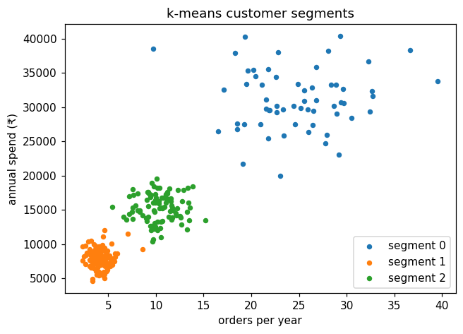

The summary table is how clusters become useful: give each segment a name ("occasional", "regular", "VIP") and a strategy. Cluster numbers themselves are arbitrary; running again with another random_state may number them differently.

Scale first. k-means uses distances, so without scaling, annual spend (thousands of rupees) would completely dominate the number of orders.

Choosing k#

With no labels, there is no "right answer" to check. Two common guides:

• Inertia (the elbow method): the total squared distance from points to their centroid. It always decreases as k grows; look for the "elbow" where adding clusters stops helping much.
• Silhouette score: how much closer each point is to its own cluster than to the next nearest one, from −1 to 1. Higher is better.

import numpy as np
from sklearn.cluster import KMeans
from sklearn.metrics import silhouette_score
from sklearn.preprocessing import StandardScaler

rng = np.random.default_rng(3)
groups = [((8000, 4), 120), ((30000, 25), 60), ((15000, 10), 100)]
X = np.vstack([np.column_stack([rng.normal(m[0], m[0] * 0.15, n), rng.normal(m[1], m[1] * 0.2, n)]) for m, n in groups])
X = StandardScaler().fit_transform(X)

for k in range(2, 7):
    km = KMeans(n_clusters=k, n_init=10, random_state=0).fit(X)
    print(f"k={k}: inertia {km.inertia_:7.1f}, silhouette {silhouette_score(X, km.labels_):.3f}")

k=2: inertia   116.6, silhouette 0.741
k=3: inertia    50.8, silhouette 0.698
k=4: inertia    35.5, silhouette 0.647
k=5: inertia    28.3, silhouette 0.650
k=6: inertia    24.6, silhouette 0.650

The inertia drops sharply from k=2 to k=3 and only slowly after that, so the elbow is at 3, matching how the data was generated. The silhouette score, though, is highest at k=2: the low- and mid-spending groups sit fairly close together, so merging them still gives well-separated clusters. The two guides disagree, which is common with real data. The final choice also depends on what is useful: here three segments with distinct strategies beat two, and five segments a marketing team can act on beat twelve they cannot.

Assigning new points#

A fitted model assigns new customers to the nearest segment with predict (after the same scaling):

import numpy as np
from sklearn.cluster import KMeans
from sklearn.pipeline import make_pipeline
from sklearn.preprocessing import StandardScaler

rng = np.random.default_rng(3)
groups = [((8000, 4), 120), ((30000, 25), 60), ((15000, 10), 100)]
X = np.vstack([np.column_stack([rng.normal(m[0], m[0] * 0.15, n), rng.normal(m[1], m[1] * 0.2, n)]) for m, n in groups])

model = make_pipeline(StandardScaler(), KMeans(n_clusters=3, n_init=10, random_state=0)).fit(X)
new_customers = np.array([[7500, 3], [32000, 27]])
print(model.predict(new_customers))
print(model.predict(np.array([[8200, 5]])) == model.predict(np.array([[7500, 3]])))

[1 0]
[ True]

The low spender joins segment 1 and the big spender joins segment 0, matching the segment averages in this run, and a similar low spender lands in the same segment.

Limits of k-means#

• You must choose k.
• It assumes roughly round, similarly sized clusters; long, curved or very uneven clusters are split badly. DBSCAN finds arbitrarily shaped clusters and marks outliers; hierarchical clustering builds a tree of clusters at every level.
• Results depend on scaling and on the starting centroids (n_init reduces this).
• It works with numeric features; categorical data needs encoding or a different method.

Common mistakes#

Practice#

import pandas as pd
from sklearn.cluster import KMeans
from sklearn.datasets import load_iris
from sklearn.preprocessing import StandardScaler

X, y = load_iris(return_X_y=True)
labels = KMeans(n_clusters=3, n_init=10, random_state=0).fit_predict(StandardScaler().fit_transform(X))
print(pd.crosstab(labels, y, rownames=["cluster"], colnames=["species"]))

species   0   1   2
cluster
0         0  39  14
1        50   0   0
2         0  11  36

Key takeaway#

Next: Principal Component Analysis (PCA).