Overfitting, Underfitting and the Bias-Variance Trade-off

Every model sits somewhere between two failures:

• Underfitting: the model is too simple to capture the pattern. It does badly on training and new data. This is high bias.
• Overfitting: the model is so flexible that it learns noise in the training data. It does very well on training data but badly on new data. This is high variance (its predictions would change a lot with a different training sample).

The goal is the sweet spot in between, and the main tool for finding it is comparing training and validation scores.

Diagnosing with two scores#

A validation curve#

A validation curve plots both scores as one hyperparameter changes model complexity. Here, the maximum depth of a decision tree:

import numpy as np
import matplotlib.pyplot as plt
from sklearn.datasets import load_breast_cancer
from sklearn.model_selection import validation_curve
from sklearn.tree import DecisionTreeClassifier

X, y = load_breast_cancer(return_X_y=True)
depths = np.arange(1, 13)
train_scores, val_scores = validation_curve(
    DecisionTreeClassifier(random_state=0), X, y,
    param_name="max_depth", param_range=depths, cv=5)

fig, ax = plt.subplots(figsize=(7, 4))
ax.plot(depths, train_scores.mean(axis=1), marker="o", label="training")
ax.plot(depths, val_scores.mean(axis=1), marker="o", label="validation")
ax.set(xlabel="max_depth", ylabel="accuracy", title="Validation curve for a decision tree")
ax.legend()
plt.show()

best = depths[val_scores.mean(axis=1).argmax()]
print("best depth by validation:", best)
for d in [1, best, 12]:
    i = d - 1
    print(f"depth {d:>2}: train {train_scores[i].mean():.3f}, validation {val_scores[i].mean():.3f}")

best depth by validation: 2
depth  1: train 0.924, validation 0.900
depth  2: train 0.952, validation 0.928
depth 12: train 1.000, validation 0.917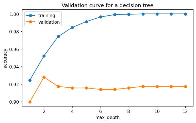

At depth 1 both scores are lower: underfitting. As depth grows, training accuracy keeps rising to a perfect score while validation accuracy stops improving; the widening gap is overfitting. The best depth is where the validation score peaks.

A learning curve#

A learning curve plots both scores as the amount of training data grows. It answers: would more data help?

import numpy as np
import matplotlib.pyplot as plt
from sklearn.datasets import load_breast_cancer
from sklearn.ensemble import RandomForestClassifier
from sklearn.model_selection import learning_curve

X, y = load_breast_cancer(return_X_y=True)
sizes, train_scores, val_scores = learning_curve(
    RandomForestClassifier(n_estimators=100, random_state=0), X, y,
    train_sizes=np.linspace(0.1, 1.0, 6), cv=5, n_jobs=-1)

fig, ax = plt.subplots(figsize=(7, 4))
ax.plot(sizes, train_scores.mean(axis=1), marker="o", label="training")
ax.plot(sizes, val_scores.mean(axis=1), marker="o", label="validation")
ax.set(xlabel="training examples", ylabel="accuracy", title="Learning curve for a random forest")
ax.legend()
plt.show()
for n, v in zip(sizes, val_scores.mean(axis=1)):
    print(n, round(v, 3))

45 0.743
127 0.924
209 0.942
291 0.956
373 0.965
455 0.963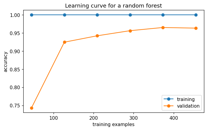

Validation accuracy rises steeply at first and then levels off around 0.96: the last two points are almost equal. More data of the same kind is therefore unlikely to help much; better features or a different model would be the next things to try. If the curve were still climbing at the right edge, collecting more data would be the obvious next step.

Fixes#

Why "trade-off"?#

Making a model more flexible lowers bias but raises variance; making it simpler does the opposite. The total error on new data is smallest somewhere in the middle. Ensembles are a way to break the trade-off partly: averaging many high-variance trees reduces variance without adding much bias, which is why random forests work so well.

Common mistakes#

Practice#

from sklearn.datasets import load_wine
from sklearn.model_selection import validation_curve
from sklearn.neighbors import KNeighborsClassifier
from sklearn.pipeline import make_pipeline
from sklearn.preprocessing import StandardScaler

X, y = load_wine(return_X_y=True)
ks = [1, 3, 5, 9, 15, 25, 45]
train, val = validation_curve(make_pipeline(StandardScaler(), KNeighborsClassifier()), X, y,
                              param_name="kneighborsclassifier__n_neighbors", param_range=ks, cv=5)
for k, t, v in zip(ks, train.mean(axis=1), val.mean(axis=1)):
    print(k, round(t, 3), round(v, 3))

1 1.0 0.95
3 0.973 0.944
5 0.975 0.949
9 0.972 0.966
15 0.972 0.955
25 0.979 0.961
45 0.965 0.961

Key takeaway#

Next: Imbalanced Data.