Machine Learning course menu

Logistic Regression in Python: Classification with Probabilities

Learn logistic regression for classification: the sigmoid function, predicting probabilities with predict_proba, the decision threshold, interpreting coefficients as odds, multi-class classification, and scaling with a pipeline.

Intermediate9 min readUpdated October 24, 2026

On this page

From a line to a probability
Training a classifier
Changing the threshold
Interpreting coefficients
More than two classes
Common mistakes
Practice
Key takeaway

Despite its name, logistic regression is a classification algorithm. It predicts the probability that an example belongs to a class (spam, fraud, will churn), and it is the standard first model for yes/no problems: fast, reliable and easy to interpret.

From a line to a probability#

Linear regression produces any number, but a probability must be between 0 and 1. Logistic regression computes a linear score and passes it through the sigmoid function, which squashes any number into that range:

Text

probability = 1 / (1 + e^(−score)),   score = intercept + w₁·x₁ + … + wₙ·xₙ

Python

import numpy as np
import matplotlib.pyplot as plt

z = np.linspace(-8, 8, 200)
sigmoid = 1 / (1 + np.exp(-z))

fig, ax = plt.subplots(figsize=(7, 3.5))
ax.plot(z, sigmoid, color="#4C72B0")
ax.axhline(0.5, color="grey", linestyle="--", linewidth=0.8)
ax.axvline(0, color="grey", linestyle="--", linewidth=0.8)
ax.set(xlabel="linear score", ylabel="probability", title="The sigmoid function")
plt.show()
print([round(float(1 / (1 + np.exp(-v))), 3) for v in [-4, -1, 0, 1, 4]])

Output

[0.018, 0.269, 0.5, 0.731, 0.982]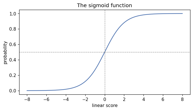

An S-shaped curve rising from near 0 at the left to near 1 at the right, crossing 0.5 where the score is 0.

A score of 0 gives a probability of 0.5; large positive scores approach 1, large negative scores approach 0.

Training a classifier#

Predicting whether a customer will buy, from minutes spent on the site and pages viewed (simulated data):

Python

import numpy as np
import pandas as pd
from sklearn.linear_model import LogisticRegression
from sklearn.model_selection import train_test_split

rng = np.random.default_rng(5)
n = 400
visits = pd.DataFrame({"minutes": rng.uniform(1, 30, n), "pages": rng.integers(1, 20, n)})
score = -6 + 0.2 * visits["minutes"] + 0.25 * visits["pages"]
visits["bought"] = (rng.random(n) < 1 / (1 + np.exp(-score))).astype(int)

X = visits[["minutes", "pages"]]
y = visits["bought"]
X_train, X_test, y_train, y_test = train_test_split(X, y, test_size=0.25, random_state=0, stratify=y)

model = LogisticRegression().fit(X_train, y_train)
print("accuracy:", round(model.score(X_test, y_test), 3))
print("coefficients:", model.coef_.round(3), "intercept:", model.intercept_.round(3))

new_visitors = pd.DataFrame({"minutes": [3, 15, 28], "pages": [2, 8, 15]})
print(model.predict_proba(new_visitors).round(3))
print(model.predict(new_visitors))

Output

accuracy: 0.84
coefficients: [[0.177 0.244]] intercept: [-5.469]
[[0.988 0.012]
 [0.704 0.296]
 [0.042 0.958]]
[0 0 1]

predict_proba returns one column per class: the probability of 0 (no purchase) and of 1 (purchase). predict returns the class with the higher probability, which means using a threshold of 0.5.

Changing the threshold#

0.5 is not always the right cut-off. If missing a buyer is cheap but a wasted discount is expensive, you might only target visitors above 0.7. Lowering the threshold catches more positives at the cost of more false alarms:

Python

import numpy as np
import pandas as pd
from sklearn.linear_model import LogisticRegression
from sklearn.model_selection import train_test_split

rng = np.random.default_rng(5)
n = 400
visits = pd.DataFrame({"minutes": rng.uniform(1, 30, n), "pages": rng.integers(1, 20, n)})
score = -6 + 0.2 * visits["minutes"] + 0.25 * visits["pages"]
visits["bought"] = (rng.random(n) < 1 / (1 + np.exp(-score))).astype(int)
X_train, X_test, y_train, y_test = train_test_split(visits[["minutes", "pages"]], visits["bought"],
                                                    test_size=0.25, random_state=0, stratify=visits["bought"])
model = LogisticRegression().fit(X_train, y_train)

proba = model.predict_proba(X_test)[:, 1]
for threshold in [0.3, 0.5, 0.7]:
    predicted = (proba >= threshold).astype(int)
    caught = ((predicted == 1) & (y_test == 1)).sum()
    flagged = predicted.sum()
    print(f"threshold {threshold}: flagged {flagged}, of which real buyers {caught} (of {y_test.sum()} buyers)")

Output

threshold 0.3: flagged 61, of which real buyers 41 (of 43 buyers)
threshold 0.5: flagged 43, of which real buyers 35 (of 43 buyers)
threshold 0.7: flagged 35, of which real buyers 30 (of 43 buyers)

Choosing the threshold is a business decision; Classification Metrics gives the tools (precision, recall, ROC curves) to make it.

Interpreting coefficients#

A positive coefficient raises the probability; a negative one lowers it. More precisely, a one-unit increase in a feature multiplies the odds (p / (1 − p)) by e^coefficient:

Python

import numpy as np

coefficients = {"minutes": 0.2, "pages": 0.25}
for feature, c in coefficients.items():
    print(feature, "odds multiplied by", round(np.exp(c), 3), "per unit")

Output

minutes odds multiplied by 1.221 per unit
pages odds multiplied by 1.284 per unit

With the true coefficients used to simulate the data, each extra page viewed multiplies the odds of buying by about 1.28 (a 28% increase in the odds).

More than two classes#

LogisticRegression also handles several classes, predicting a probability for each. Scaling the features first helps the solver converge:

Python

from sklearn.datasets import load_wine
from sklearn.linear_model import LogisticRegression
from sklearn.model_selection import train_test_split
from sklearn.pipeline import make_pipeline
from sklearn.preprocessing import StandardScaler

X, y = load_wine(return_X_y=True)
X_train, X_test, y_train, y_test = train_test_split(X, y, test_size=0.25, random_state=0, stratify=y)
model = make_pipeline(StandardScaler(), LogisticRegression()).fit(X_train, y_train)
print("accuracy:", round(model.score(X_test, y_test), 3))
print(model.predict_proba(X_test[:2]).round(3))

Output

accuracy: 1.0
[[0.001 0.001 0.997]
 [0.867 0.132 0.001]]

Each row of probabilities sums to 1 across the three wine classes.

Common mistakes#

Practice#

Practice exercise

On the breast cancer dataset (load_breast_cancer(return_X_y=True)), split 75/25 with stratify and random_state=3, fit a scaled logistic regression, and print the test accuracy and how many test cases have a predicted probability between 0.3 and 0.7 (the uncertain ones).

Show hint

make_pipeline(StandardScaler(), LogisticRegression()); then proba = model.predict_proba(X_test)[:, 1] and count (proba > 0.3) & (proba < 0.7).

Show solution

Python

from sklearn.datasets import load_breast_cancer
from sklearn.linear_model import LogisticRegression
from sklearn.model_selection import train_test_split
from sklearn.pipeline import make_pipeline
from sklearn.preprocessing import StandardScaler

X, y = load_breast_cancer(return_X_y=True)
X_train, X_test, y_train, y_test = train_test_split(X, y, test_size=0.25, stratify=y, random_state=3)
model = make_pipeline(StandardScaler(), LogisticRegression()).fit(X_train, y_train)
proba = model.predict_proba(X_test)[:, 1]
print(round(model.score(X_test, y_test), 3))
print(int(((proba > 0.3) & (proba < 0.7)).sum()), "uncertain cases of", len(proba))

Output

0.986
5 uncertain cases of 143

In a real medical setting, uncertain cases like these are the ones to send for a specialist's review.

Key takeaway#

Next: Classification Metrics.

Finished this lesson?

Machine LearningClassification Metrics: Confusion Matrix, Precision, Recall, F1 and ROC AUCEvaluate classifiers properly: why accuracy misleads on imbalanced data, the confusion matrix, precision, recall, F1 score, classification_report, the precision-recall trade-off, ROC curves and AUC, with scikit-learn.Intermediate9 min read Machine LearningLinear Regression in Python with scikit-learn (Explained Simply)Learn linear regression: fitting a straight line to data, the slope and intercept, how least squares works, training LinearRegression in scikit-learn, interpreting coefficients, making predictions and checking residuals.Beginner6 min read Machine Learningscikit-learn Pipelines and ColumnTransformer ExplainedCombine preprocessing and models into one object with scikit-learn Pipeline and ColumnTransformer: different steps for numeric and categorical columns, preventing data leakage, cross-validating and tuning whole pipelines, and predicting on raw data.Intermediate9 min read

From a line to a probability#

Training a classifier#

Changing the threshold#

Interpreting coefficients#

More than two classes#

Common mistakes#

Practice#

Key takeaway#

Related lessons