Correlation in Python: Pearson, Spearman and Correlation Matrices

Correlation measures how strongly two numeric variables move together. Do customers who visit more often spend more? Do longer delivery times mean lower ratings? The correlation coefficient r answers with a single number from −1 to +1:

Look first: a scatter plot#

import numpy as np
import pandas as pd
import matplotlib.pyplot as plt

rng = np.random.default_rng(1)
visits = rng.integers(1, 30, size=60)
spend = 150 * visits + rng.normal(0, 600, size=60)
delivery = rng.uniform(15, 60, size=60)
rating = 5.5 - 0.05 * delivery + rng.normal(0, 0.3, size=60)

fig, axes = plt.subplots(1, 2, figsize=(10, 4))
axes[0].scatter(visits, spend, color="#4C72B0")
axes[0].set(xlabel="Visits per month", ylabel="Spend (₹)", title="Positive relationship")
axes[1].scatter(delivery, rating, color="#C44E52")
axes[1].set(xlabel="Delivery time (min)", ylabel="Rating", title="Negative relationship")
plt.tight_layout()
plt.show()

df = pd.DataFrame({"visits": visits, "spend": spend, "delivery": delivery, "rating": rating})
print(round(df["visits"].corr(df["spend"]), 2))
print(round(df["delivery"].corr(df["rating"]), 2))

0.93
-0.87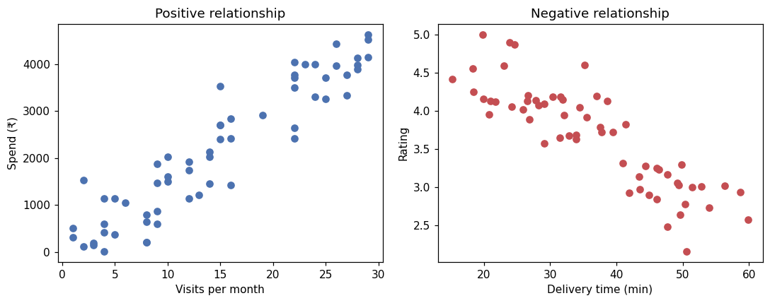

The correlation matrix#

df.corr() computes r for every pair of numeric columns at once:

import numpy as np
import pandas as pd

rng = np.random.default_rng(1)
visits = rng.integers(1, 30, size=60)
spend = 150 * visits + rng.normal(0, 600, size=60)
delivery = rng.uniform(15, 60, size=60)
rating = 5.5 - 0.05 * delivery + rng.normal(0, 0.3, size=60)
df = pd.DataFrame({"visits": visits, "spend": spend, "delivery": delivery, "rating": rating})
print(df.corr().round(2))

          visits  spend  delivery  rating
visits      1.00   0.93     -0.11    0.13
spend       0.93   1.00     -0.15    0.14
delivery   -0.11  -0.15      1.00   -0.87
rating      0.13   0.14     -0.87    1.00

The diagonal is always 1 (every column correlates perfectly with itself) and the matrix is symmetric. Pairs that were simulated independently, like visits and rating, are small (between −0.15 and 0.15). They are not exactly 0 because, with only 60 points, chance alone produces small correlations. A heatmap of this matrix is shown in the seaborn lesson.

Pearson and Spearman#

The default, Pearson correlation, measures linear relationships and is sensitive to outliers. Spearman correlation works on the ranks of the values, so it captures any steadily increasing (or decreasing) relationship and resists outliers:

import pandas as pd

x = pd.Series([1, 2, 3, 4, 5, 6, 7, 8])
curved = x ** 3                                   # always increasing, not a straight line
with_outlier = pd.Series([2, 4, 5, 4, 6, 7, 8, 100])

print(round(x.corr(curved), 3), round(x.corr(curved, method="spearman"), 3))
print(round(x.corr(with_outlier), 3), round(x.corr(with_outlier, method="spearman"), 3))

0.932 1.0
0.62 0.958

The cubic relationship is perfectly monotonic, so Spearman gives exactly 1 while Pearson is lower. One extreme value changes Pearson's r far more than Spearman's.

r near 0 does not mean "unrelated"#

Correlation only measures straight-line (Pearson) or monotonic (Spearman) relationships. A U-shaped relationship can have r ≈ 0:

import numpy as np

x = np.linspace(-3, 3, 61)
y = x ** 2
print(round(np.corrcoef(x, y)[0, 1], 3))

0.0

y is completely determined by x, yet r is 0. Always plot the data.

Correlation is not causation#

Ice cream sales and drowning incidents are positively correlated, because both rise in hot weather. A third variable (a confounder) drives both. Correlation can also be coincidence in small samples, or the cause can run the other way. To claim that one thing causes another, you need a controlled experiment such as an A/B test, or careful causal analysis.

Common mistakes#

Practice#

import pandas as pd

df = pd.DataFrame({"hours": [2, 4, 5, 3, 8, 7, 1, 6], "score": [55, 65, 70, 58, 92, 85, 50, 76]})
print(round(df["hours"].corr(df["score"]), 3), round(df["hours"].corr(df["score"], method="spearman"), 3))

more = pd.concat([df, pd.DataFrame({"hours": [9], "score": [40]})], ignore_index=True)
print(round(more["hours"].corr(more["score"]), 3), round(more["hours"].corr(more["score"], method="spearman"), 3))

0.992 1.0
0.369 0.4

Key takeaway#

Next: Probability Basics.