Python for Data course menu
matplotlib Subplots and Styling: Multiple Charts, Formatting and Themes
Put several charts in one figure with plt.subplots, share axes, build small multiples, format axis ticks as currency or percentages, remove chart clutter, use built-in styles, and choose accessible colours.
On this page
Real reports usually need several related charts, clean formatting and consistent colours. This lesson covers the matplotlib tools for that.
A grid of charts#
plt.subplots(rows, cols) returns a Figure and an array of Axes. Index it like a NumPy array:
import numpy as np
import matplotlib.pyplot as plt

rng = np.random.default_rng(2)
months = np.arange(1, 13)
revenue = 100 + 8 * months + rng.normal(0, 10, 12)
customers = 50 + 5 * months + rng.normal(0, 6, 12)
order_value = rng.normal(800, 120, 300)
channels = {"Web": 52, "App": 33, "Store": 15}

fig, axes = plt.subplots(2, 2, figsize=(10, 7))
axes[0, 0].plot(months, revenue, marker="o")
axes[0, 0].set_title("Revenue (₹ thousands)")
axes[0, 1].plot(months, customers, marker="o", color="#55A868")
axes[0, 1].set_title("New customers")
axes[1, 0].hist(order_value, bins=25, color="#8172B3", edgecolor="white")
axes[1, 0].set_title("Order value distribution (₹)")
axes[1, 1].bar(list(channels), list(channels.values()), color="#DD8452")
axes[1, 1].set_title("Orders by channel (%)")
fig.suptitle("Shop dashboard, 2026", fontsize=14)
fig.tight_layout()
plt.show()
print(axes.shape)(2, 2)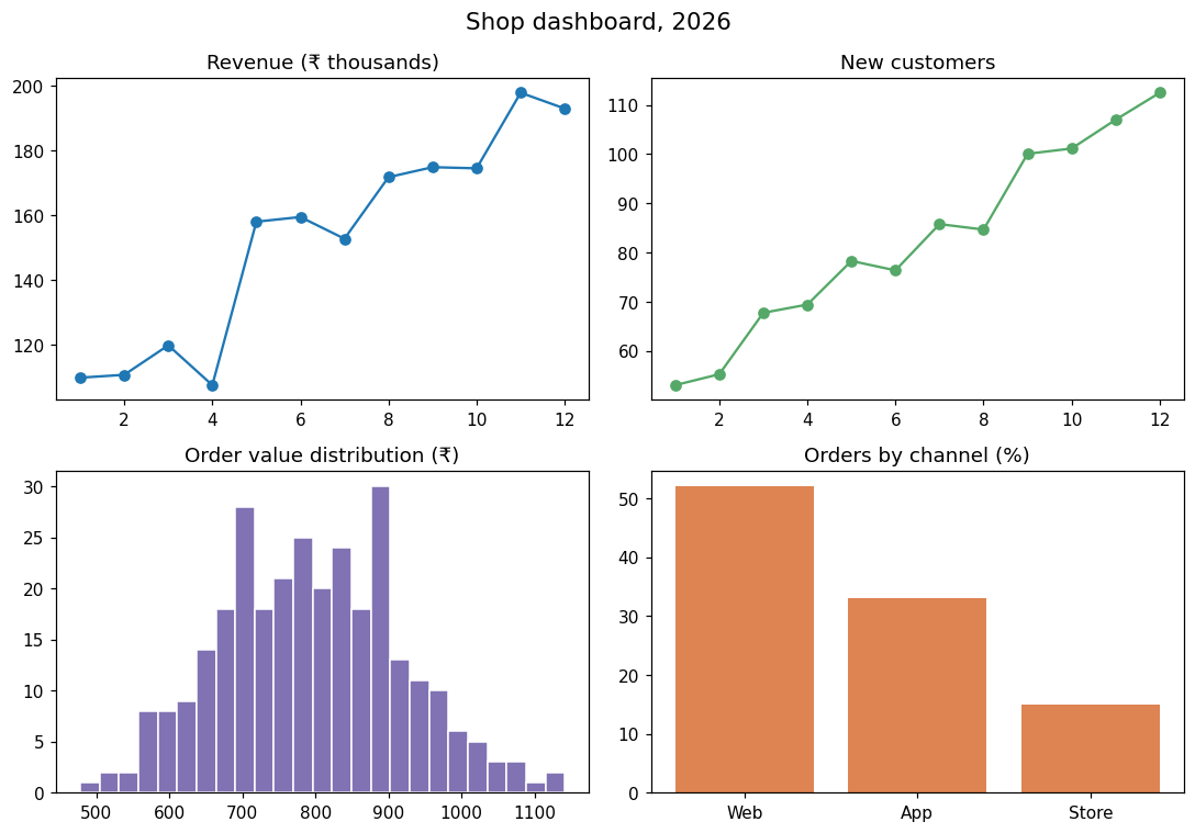
fig.suptitle titles the whole figure, and tight_layout() spaces the charts so titles and labels do not overlap.
Small multiples with shared axes#
To compare the same measure across groups, draw one small chart per group with shared axes, so the scales are identical:
import numpy as np
import matplotlib.pyplot as plt

rng = np.random.default_rng(6)
weeks = np.arange(1, 13)
stores = {
    "Mumbai": 200 + 10 * weeks + rng.normal(0, 15, 12),
    "Delhi": 180 + 4 * weeks + rng.normal(0, 15, 12),
    "Pune": 120 + 12 * weeks + rng.normal(0, 15, 12),
    "Chennai": 150 - 2 * weeks + rng.normal(0, 15, 12),
}

fig, axes = plt.subplots(1, 4, figsize=(12, 3), sharey=True)
for ax, (store, sales) in zip(axes, stores.items()):
    ax.plot(weeks, sales, color="#4C72B0")
    ax.set_title(store)
    ax.set_xlabel("Week")
axes[0].set_ylabel("Sales")
fig.tight_layout()
plt.show()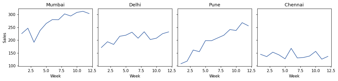
Because the y axes are shared, it is immediately clear that Chennai is declining and Pune is growing fastest. Separate scales would hide that.
Formatting ticks: currency and percentages#
import matplotlib.pyplot as plt
from matplotlib.ticker import FuncFormatter, PercentFormatter

months = ["Jan", "Feb", "Mar", "Apr", "May", "Jun"]
revenue = [1_200_000, 1_350_000, 1_280_000, 1_520_000, 1_610_000, 1_740_000]
conversion = [0.031, 0.034, 0.029, 0.037, 0.041, 0.044]

fig, (ax1, ax2) = plt.subplots(1, 2, figsize=(10, 3.5))
ax1.bar(months, revenue, color="#4C72B0")
ax1.yaxis.set_major_formatter(FuncFormatter(lambda v, _: f"₹{v / 100_000:.0f}L"))
ax1.set_title("Revenue")
ax2.plot(months, conversion, marker="o", color="#C44E52")
ax2.yaxis.set_major_formatter(PercentFormatter(xmax=1, decimals=1))
ax2.set_ylim(0, 0.05)
ax2.set_title("Conversion rate")
fig.tight_layout()
plt.show()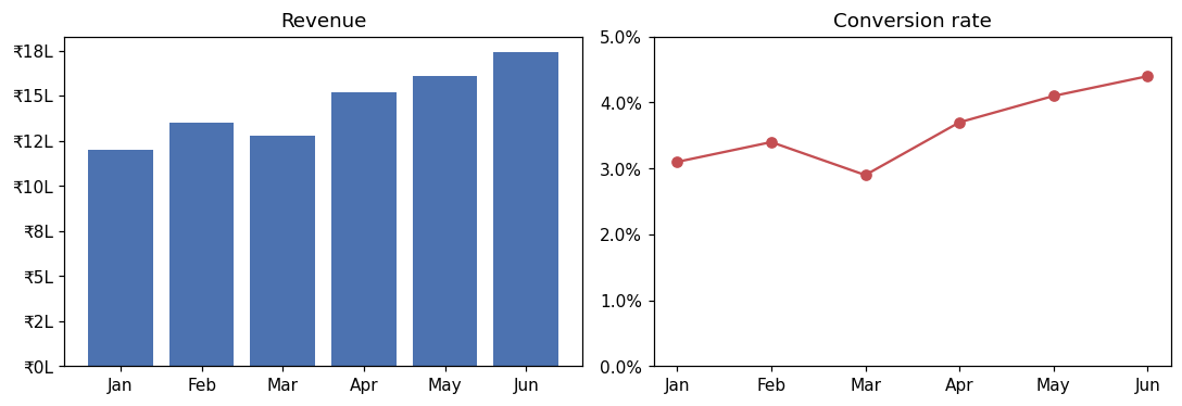
FuncFormatter takes any function of the tick value; PercentFormatter(xmax=1) treats 1.0 as 100%.
Removing clutter#
Less ink makes the data stand out. Remove the top and right borders, lighten the gridlines and label lines directly instead of using a legend:
import matplotlib.pyplot as plt

years = [2021, 2022, 2023, 2024, 2025, 2026]
python = [48, 52, 57, 61, 66, 70]
java = [40, 38, 37, 35, 34, 33]

fig, ax = plt.subplots(figsize=(7, 4))
ax.plot(years, python, color="#4C72B0", linewidth=2.5)
ax.plot(years, java, color="#A1A9B3", linewidth=2)
ax.text(2026.1, python[-1], "Python", color="#4C72B0", va="center")
ax.text(2026.1, java[-1], "Java", color="#666666", va="center")
ax.spines[["top", "right"]].set_visible(False)
ax.grid(axis="y", alpha=0.25)
ax.set_ylim(0, 80)
ax.set_title("Share of new course enrolments (%), illustrative data", loc="left")
fig.tight_layout()
plt.show()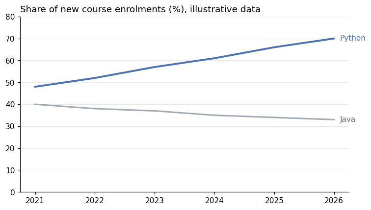
The numbers in this example are made up for illustration, and the title says so. Real charts should always state their data source.
Styles and colours#
matplotlib has built-in styles that change the look of every chart at once:
import matplotlib.pyplot as plt

print(len(plt.style.available) > 10)
print([s for s in plt.style.available if s in ("ggplot", "fivethirtyeight", "seaborn-v0_8-whitegrid", "tableau-colorblind10")])True
['fivethirtyeight', 'ggplot', 'seaborn-v0_8-whitegrid', 'tableau-colorblind10']Use one with plt.style.use("seaborn-v0_8-whitegrid") at the top of a notebook. For colours:
- Use a colourblind-friendly palette (such as
tableau-colorblind10, or seaborn's"colorblind"palette); about 1 in 12 men has some form of colour vision deficiency. - Use one strong colour for what matters and grey for the rest.
- Use sequential colours (light to dark) for ordered values and distinct hues only for unrelated categories.
Common mistakes#
Practice#
Practice exercise
Make a 1 × 2 figure: on the left, a bar chart of monthly sign-ups [320, 410, 380, 520] for Jan–Apr; on the right, the month-over-month growth in percent as a line, with the y axis formatted as percentages. Remove the top and right borders on both. Print the growth values (1 decimal).
Show hint
Growth = (this month − last month) / last month. PercentFormatter(xmax=100) formats values already in percent.
Show solution
import matplotlib.pyplot as plt
from matplotlib.ticker import PercentFormatter

months = ["Jan", "Feb", "Mar", "Apr"]
signups = [320, 410, 380, 520]
growth = [(b - a) / a * 100 for a, b in zip(signups, signups[1:])]

fig, (left, right) = plt.subplots(1, 2, figsize=(10, 3.5))
left.bar(months, signups, color="#4C72B0")
left.set_title("Sign-ups")
right.plot(months[1:], growth, marker="o", color="#C44E52")
right.axhline(0, color="grey", linewidth=0.8)
right.yaxis.set_major_formatter(PercentFormatter(xmax=100))
right.set_title("Month-over-month growth")
for ax in (left, right):
    ax.spines[["top", "right"]].set_visible(False)
fig.tight_layout()
plt.show()
print([round(g, 1) for g in growth])[28.1, -7.3, 36.8]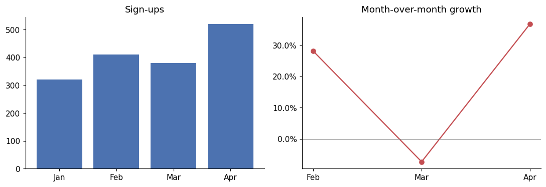
Key takeaway#
Finished this lesson?