Python for Data course menu
seaborn Tutorial: Statistical Charts in a Few Lines of Python
Make statistical charts with seaborn from pandas DataFrames: bar plots with averages, box and violin plots, histograms with KDE, scatter plots with hue, regression lines, correlation heatmaps and faceted plots.
On this page
seaborn builds on matplotlib and works directly with pandas DataFrames: you name the columns, and it handles grouping, colours, legends and statistical summaries. Charts that need ten lines of matplotlib often take one line of seaborn.
All examples use this simulated restaurant dataset (in long format: one row per bill):
import numpy as np
import pandas as pd

rng = np.random.default_rng(12)
n = 240
bills = pd.DataFrame({
    "day": rng.choice(["Thu", "Fri", "Sat", "Sun"], n, p=[0.2, 0.2, 0.3, 0.3]),
    "time": rng.choice(["Lunch", "Dinner"], n, p=[0.35, 0.65]),
    "size": rng.integers(1, 7, n),
})
bills["total"] = (180 * bills["size"] + rng.normal(0, 120, n)
                  + np.where(bills["time"] == "Dinner", 150, 0)).round(0).clip(lower=120)
bills["tip"] = (bills["total"] * rng.uniform(0.05, 0.2, n)).round(0)
print(bills.head())
print(bills.shape) day time size total tip
0 Fri Lunch 1 120.0 13.0
1 Sun Lunch 2 224.0 26.0
2 Thu Lunch 3 477.0 25.0
3 Thu Dinner 3 672.0 42.0
4 Fri Lunch 5 953.0 119.0
(240, 5)Comparing groups: barplot and boxplot#
sns.barplot shows the mean of a column for each category, with an error bar for its uncertainty. sns.boxplot shows each group's whole distribution:
import numpy as np
import pandas as pd
import seaborn as sns
import matplotlib.pyplot as plt

rng = np.random.default_rng(12)
n = 240
bills = pd.DataFrame({
    "day": rng.choice(["Thu", "Fri", "Sat", "Sun"], n, p=[0.2, 0.2, 0.3, 0.3]),
    "time": rng.choice(["Lunch", "Dinner"], n, p=[0.35, 0.65]),
    "size": rng.integers(1, 7, n),
})
bills["total"] = (180 * bills["size"] + rng.normal(0, 120, n)
                  + np.where(bills["time"] == "Dinner", 150, 0)).round(0).clip(lower=120)

order = ["Thu", "Fri", "Sat", "Sun"]
fig, axes = plt.subplots(1, 2, figsize=(11, 4))
sns.barplot(data=bills, x="day", y="total", order=order, ax=axes[0])
axes[0].set_title("Average bill by day")
sns.boxplot(data=bills, x="time", y="total", hue="time", ax=axes[1])
axes[1].set_title("Bills at lunch and dinner")
fig.tight_layout()
plt.show()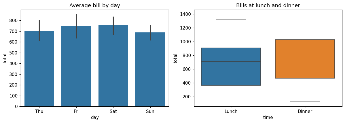
Notice there is no grouping code: seaborn computes the means and quartiles itself. The error bars are 95% confidence intervals for the mean by default.
Distributions: histplot with KDE#
import numpy as np
import pandas as pd
import seaborn as sns
import matplotlib.pyplot as plt

rng = np.random.default_rng(12)
n = 240
bills = pd.DataFrame({
    "day": rng.choice(["Thu", "Fri", "Sat", "Sun"], n, p=[0.2, 0.2, 0.3, 0.3]),
    "time": rng.choice(["Lunch", "Dinner"], n, p=[0.35, 0.65]),
    "size": rng.integers(1, 7, n),
})
bills["total"] = (180 * bills["size"] + rng.normal(0, 120, n)
                  + np.where(bills["time"] == "Dinner", 150, 0)).round(0).clip(lower=120)

fig, ax = plt.subplots(figsize=(7, 4))
sns.histplot(data=bills, x="total", hue="time", kde=True, bins=20, ax=ax)
ax.set_title("Bill totals by meal")
plt.show()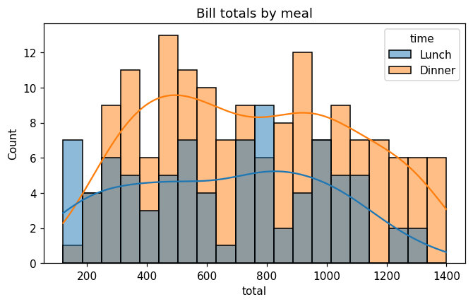
kde=True adds a smooth kernel density estimate curve over the histogram.
Relationships: scatterplot and regplot#
import numpy as np
import pandas as pd
import seaborn as sns
import matplotlib.pyplot as plt

rng = np.random.default_rng(12)
n = 240
bills = pd.DataFrame({
    "day": rng.choice(["Thu", "Fri", "Sat", "Sun"], n, p=[0.2, 0.2, 0.3, 0.3]),
    "time": rng.choice(["Lunch", "Dinner"], n, p=[0.35, 0.65]),
    "size": rng.integers(1, 7, n),
})
bills["total"] = (180 * bills["size"] + rng.normal(0, 120, n)
                  + np.where(bills["time"] == "Dinner", 150, 0)).round(0).clip(lower=120)
bills["tip"] = (bills["total"] * rng.uniform(0.05, 0.2, n)).round(0)

fig, axes = plt.subplots(1, 2, figsize=(11, 4))
sns.scatterplot(data=bills, x="total", y="tip", hue="time", ax=axes[0])
axes[0].set_title("Tip vs bill, coloured by meal")
sns.regplot(data=bills, x="size", y="total", ax=axes[1], x_jitter=0.15)
axes[1].set_title("Bill vs party size, with trend line")
fig.tight_layout()
plt.show()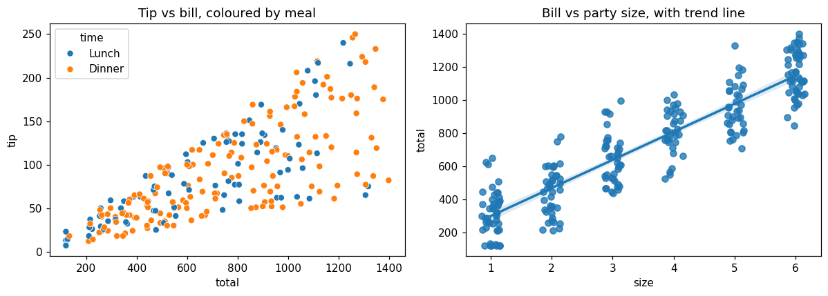
hue colours points by a category; regplot adds a fitted straight line with a shaded confidence band. x_jitter spreads overlapping points that share the same party size.
Correlation heatmap#
A heatmap is the standard way to show a correlation matrix:
import numpy as np
import pandas as pd
import seaborn as sns
import matplotlib.pyplot as plt

rng = np.random.default_rng(12)
n = 240
bills = pd.DataFrame({"size": rng.integers(1, 7, n)})
bills["total"] = (180 * bills["size"] + rng.normal(0, 120, n)).round(0).clip(lower=120)
bills["tip"] = (bills["total"] * rng.uniform(0.05, 0.2, n)).round(0)
bills["wait_min"] = rng.normal(20, 6, n).round(0)

corr = bills.corr()
fig, ax = plt.subplots(figsize=(5, 4))
sns.heatmap(corr, annot=True, fmt=".2f", cmap="RdBu_r", vmin=-1, vmax=1, ax=ax)
ax.set_title("Correlation matrix")
plt.show()
print(corr.round(2)) size total tip wait_min
size 1.00 0.93 0.71 0.02
total 0.93 1.00 0.76 0.01
tip 0.71 0.76 1.00 0.07
wait_min 0.02 0.01 0.07 1.00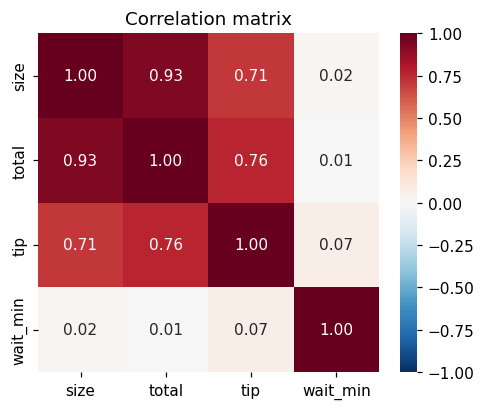
annot=True writes the values; fixing vmin=-1, vmax=1 with a diverging palette (RdBu_r) makes the colour meaning consistent across charts.
Facets: one chart per group#
Figure-level functions such as sns.relplot, sns.displot and sns.catplot can split the data into a grid of charts with col and row:
import numpy as np
import pandas as pd
import seaborn as sns
import matplotlib.pyplot as plt

rng = np.random.default_rng(12)
n = 240
bills = pd.DataFrame({
    "time": rng.choice(["Lunch", "Dinner"], n, p=[0.35, 0.65]),
    "size": rng.integers(1, 7, n),
})
bills["total"] = (180 * bills["size"] + rng.normal(0, 120, n)
                  + np.where(bills["time"] == "Dinner", 150, 0)).round(0).clip(lower=120)
bills["tip"] = (bills["total"] * rng.uniform(0.05, 0.2, n)).round(0)

grid = sns.relplot(data=bills, x="total", y="tip", col="time", height=3.5, aspect=1.2)
grid.set_titles("{col_name}")
plt.show()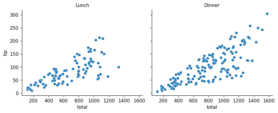
Common mistakes#
Practice#
Practice exercise
Using the bills data from the first example, draw a sns.countplot of how many bills there were on each day (in the order Thu, Fri, Sat, Sun), and print the counts per day.
Show hint
sns.countplot(data=bills, x="day", order=[...]) counts rows; bills["day"].value_counts() gives the same numbers.
Show solution
import numpy as np
import pandas as pd
import seaborn as sns
import matplotlib.pyplot as plt

rng = np.random.default_rng(12)
n = 240
bills = pd.DataFrame({
    "day": rng.choice(["Thu", "Fri", "Sat", "Sun"], n, p=[0.2, 0.2, 0.3, 0.3]),
    "time": rng.choice(["Lunch", "Dinner"], n, p=[0.35, 0.65]),
    "size": rng.integers(1, 7, n),
})

order = ["Thu", "Fri", "Sat", "Sun"]
fig, ax = plt.subplots(figsize=(6, 3.5))
sns.countplot(data=bills, x="day", order=order, ax=ax)
ax.set_title("Bills per day")
plt.show()
print(bills["day"].value_counts().reindex(order))day
Thu 56
Fri 38
Sat 68
Sun 78
Name: count, dtype: int64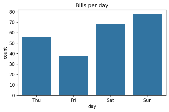
Key takeaway#
Finished this lesson?