Python for Data course menu
matplotlib Tutorial for Beginners: Line Charts, Labels and Saving Figures
Learn matplotlib basics: the Figure and Axes objects, drawing line charts, titles, axis labels and legends, markers and colours, axis limits, gridlines, and saving charts as PNG files.
On this page
matplotlib is Python's main plotting library. seaborn and pandas' own plotting are built on top of it, so knowing its basics lets you adjust any chart.
Figure and Axes#
Every chart has two key objects:
- a Figure: the whole image (the canvas);
- one or more Axes: the plotting areas inside it, each with its own x and y axis.
The recommended way to start is plt.subplots(), which creates both:
import matplotlib.pyplot as plt

months = ["Jan", "Feb", "Mar", "Apr", "May", "Jun"]
revenue = [120, 95, 140, 160, 130, 175]

fig, ax = plt.subplots(figsize=(7, 4))
ax.plot(months, revenue)
ax.set_title("Monthly revenue")
ax.set_xlabel("Month")
ax.set_ylabel("Revenue (₹ thousands)")
plt.show()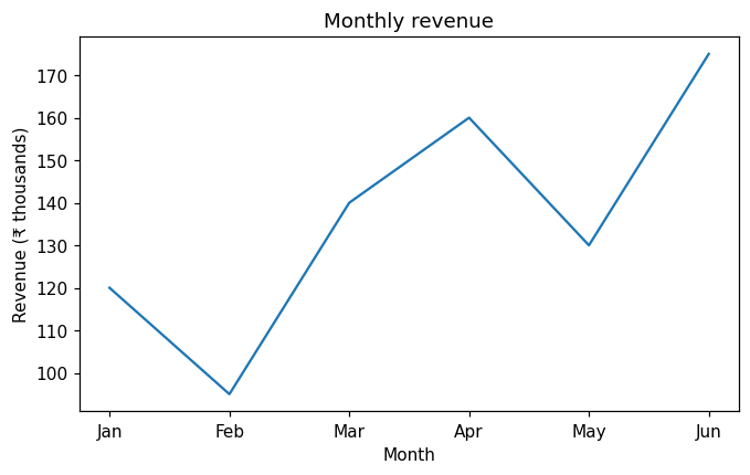
figsize is the width and height in inches. In a Jupyter notebook, plt.show() is optional (the chart appears automatically at the end of the cell); in a script it opens a window.
Several lines, markers and a legend#
import matplotlib.pyplot as plt

months = ["Jan", "Feb", "Mar", "Apr", "May", "Jun"]
north = [120, 95, 140, 160, 130, 175]
south = [90, 110, 105, 125, 150, 145]

fig, ax = plt.subplots(figsize=(7, 4))
ax.plot(months, north, marker="o", color="#4C72B0", label="North")
ax.plot(months, south, marker="s", linestyle="--", color="#DD8452", label="South")
ax.set_title("Revenue by region")
ax.set_ylabel("Revenue (₹ thousands)")
ax.set_ylim(0, 200)                 # start the y axis at zero
ax.grid(axis="y", alpha=0.3)
ax.legend()
plt.show()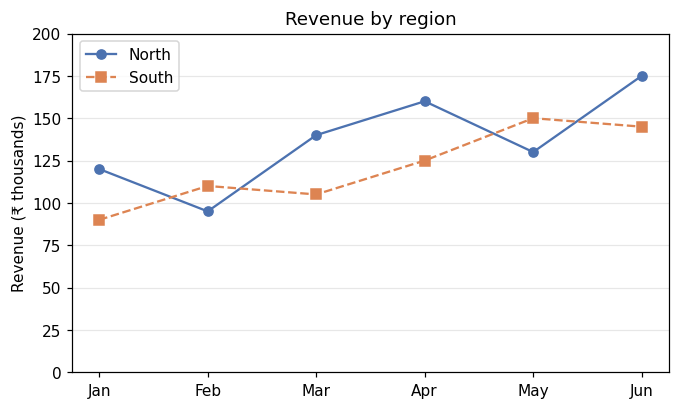
markerdraws a symbol at each point;linestyle="--"makes a dashed line.labelnames a line;ax.legend()shows the names.ax.set_ylim(0, 200)fixes the axis range. Starting at 0 avoids exaggerating differences.
Annotating a point#
Point readers to what matters with annotate:
import matplotlib.pyplot as plt

months = ["Jan", "Feb", "Mar", "Apr", "May", "Jun"]
revenue = [120, 95, 140, 160, 130, 175]
best = revenue.index(max(revenue))

fig, ax = plt.subplots(figsize=(7, 4))
ax.plot(months, revenue, marker="o")
ax.annotate(f"Best month: {max(revenue)}", xy=(best, max(revenue)),
            xytext=(best - 2.5, max(revenue) - 10),
            arrowprops={"arrowstyle": "->"})
ax.set_title("Monthly revenue")
ax.set_ylim(0, 200)
plt.show()
print("best month:", months[best])best month: Jun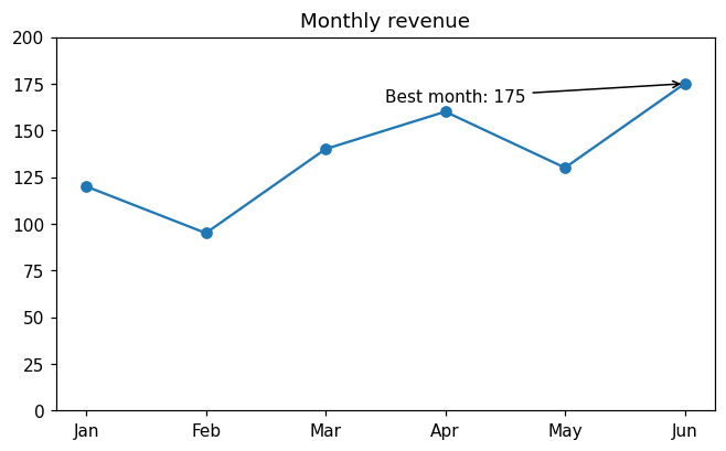
With text labels on the x axis, the positions are 0, 1, 2, …, which is why xy uses the index best.
Saving a chart#
import matplotlib.pyplot as plt

fig, ax = plt.subplots(figsize=(6, 3))
ax.bar(["A", "B", "C"], [5, 8, 3])
fig.savefig("chart.png", dpi=150, bbox_inches="tight")
plt.close(fig)

import os
print(os.path.exists("chart.png"), os.path.getsize("chart.png") > 0)True Truedpi(dots per inch) sets the resolution; 150 to 300 suits reports.bbox_inches="tight"trims empty margins so labels are not cut off.- Save as
.svgor.pdffor sharp vector graphics in documents. plt.close(fig)frees the memory when you create many charts in a loop.
Two styles of matplotlib code#
You will see two styles online:
import matplotlib.pyplot as plt

# "pyplot" style: functions act on the current chart
plt.plot([1, 2, 3], [4, 6, 5])
plt.title("pyplot style")
plt.close()

# object-oriented style: call methods on an Axes
fig, ax = plt.subplots()
ax.plot([1, 2, 3], [4, 6, 5])
ax.set_title("object-oriented style")
plt.close(fig)
print("both styles ran")both styles ranThey draw the same thing. The object-oriented style (fig, ax = plt.subplots(), then ax.something) is clearer once you have more than one chart, and it is what this course uses. Note the different method names: plt.title but ax.set_title.
Common mistakes#
Practice#
Practice exercise
Plot weekly website visitors [820, 910, 870, 1050, 1200, 1150, 1320] for weeks 1 to 7 as a line with circle markers. Add a title, axis labels, a y axis starting at 0, and a horizontal dashed line at the average (use ax.axhline). Print the average.
Show hint
ax.axhline(y=value, linestyle="--", color="grey", label="average") draws a horizontal line across the chart.
Show solution
import matplotlib.pyplot as plt

weeks = range(1, 8)
visitors = [820, 910, 870, 1050, 1200, 1150, 1320]
average = sum(visitors) / len(visitors)

fig, ax = plt.subplots(figsize=(7, 4))
ax.plot(weeks, visitors, marker="o", label="visitors")
ax.axhline(y=average, linestyle="--", color="grey", label="average")
ax.set(title="Weekly visitors", xlabel="Week", ylabel="Visitors", ylim=(0, 1500))
ax.legend()
plt.show()
print(round(average, 1))1045.7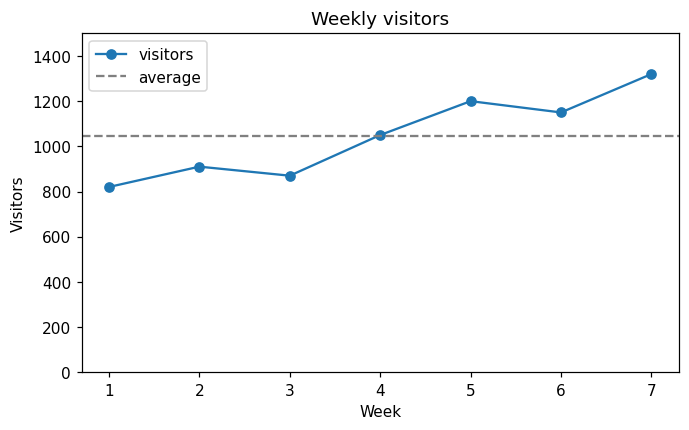
ax.set(...) sets several properties in one call.
Key takeaway#
Next: Choosing the Right Chart.
Finished this lesson?