Python for Data course menu
Exploratory Data Analysis (EDA) in Python: A Complete Project
A complete exploratory data analysis project with pandas, matplotlib and seaborn: load an e-commerce customer dataset, inspect it, clean missing values, duplicates, messy text and outliers, answer business questions, visualise findings and write conclusions.
On this page
This project walks through a full exploratory data analysis (EDA): the first, open-ended look at a new dataset to understand it, clean it and find the interesting patterns. Follow along in a Jupyter notebook and run each step.
The scenario: an online store wants to understand its customers. For each customer we have their city, age, signup channel, number of orders in the last year, total spend and whether they are a member of the loyalty programme. Questions to answer:
- What does a typical customer look like?
- Which cities and signup channels bring the most valuable customers?
- Do loyalty members spend more?
Step 1: Create the dataset#
Real projects start with a file you were given. To make this project reproducible, the code below generates a realistic dataset (with the kinds of problems real data has) and saves it as customers.csv. Run it once, then treat the file as if someone handed it to you.
import numpy as np
import pandas as pd

rng = np.random.default_rng(2026)
n = 500
cities = rng.choice(["Mumbai", "Delhi", "Bengaluru", "Pune", "Chennai"], n, p=[0.28, 0.25, 0.22, 0.13, 0.12])
channel = rng.choice(["search", "social", "referral"], n, p=[0.5, 0.3, 0.2])
member = rng.random(n) < 0.35
orders = rng.poisson(lam=np.where(member, 9, 5))
spend = (orders * rng.normal(900, 150, n) + np.where(channel == "referral", 1500, 0)).round(0).clip(min=0)
age = rng.normal(34, 9, n).round(0).clip(18, 70)

df = pd.DataFrame({
    "customer_id": np.arange(1001, 1001 + n),
    "city": cities, "age": age, "channel": channel,
    "orders": orders, "spend": spend, "member": np.where(member, "yes", "no"),
})
# real-world messiness
df.loc[rng.choice(n, 25, replace=False), "age"] = np.nan
df.loc[rng.choice(n, 40, replace=False), "city"] = df["city"].str.lower()
df.loc[rng.choice(n, 15, replace=False), "city"] = " " + df["city"] + " "
df.loc[7, "spend"] = 950000                      # a data entry error
df = pd.concat([df, df.iloc[[10, 20, 30]]], ignore_index=True)   # duplicated rows
df.to_csv("customers.csv", index=False)
print(df.shape)(503, 7)Step 2: Load and inspect#
import pandas as pd

df = pd.read_csv("customers.csv")
print(df.head())
df.info() customer_id city age channel orders spend member
0 1001 mumbai 27.0 referral 5 7055.0 no
1 1002 Bengaluru 24.0 search 8 5989.0 yes
2 1003 Delhi 40.0 referral 3 4623.0 no
3 1004 Delhi 28.0 search 2 2203.0 no
4 1005 Delhi 29.0 search 11 11141.0 no
<class 'pandas.core.frame.DataFrame'>
RangeIndex: 503 entries, 0 to 502
Data columns (total 7 columns):
# Column Non-Null Count Dtype
--- ------ -------------- -----
0 customer_id 503 non-null int64
1 city 503 non-null object
2 age 477 non-null float64
3 channel 503 non-null object
4 orders 503 non-null int64
5 spend 503 non-null float64
6 member 503 non-null object
dtypes: float64(2), int64(2), object(3)
memory usage: 27.6+ KBinfo() already shows two issues: age has missing values, and customer_id should be unique. Look further:
import pandas as pd

df = pd.read_csv("customers.csv")
print(df.describe().round(1))
print(df["city"].value_counts())
print("duplicate rows:", df.duplicated().sum()) customer_id age orders spend
count 503.0 477.0 503.0 503.0
mean 1249.1 34.0 6.5 8103.4
std 145.1 9.3 3.1 42187.8
min 1001.0 18.0 1.0 718.0
25% 1123.5 27.0 4.0 3959.0
50% 1249.0 34.0 6.0 5758.0
75% 1374.5 41.0 8.0 8107.0
max 1500.0 65.0 18.0 950000.0
city
Delhi 120
Mumbai 117
Bengaluru 103
Chennai 55
Pune 54
delhi 14
mumbai 11
chennai 5
Bengaluru 5
bengaluru 5
pune 4
Delhi 4
Mumbai 3
Chennai 2
delhi 1
Name: count, dtype: int64
duplicate rows: 3Three problems stand out:
- Spend has an extreme maximum far above the 75th percentile: likely the data entry error.
- City names are inconsistent: the same city appears with different capitalisation and stray spaces.
- There are duplicate rows.
Step 3: Clean#
import pandas as pd

df = pd.read_csv("customers.csv")
before = len(df)

df = df.drop_duplicates()
df["city"] = df["city"].str.strip().str.title()

q1, q3 = df["spend"].quantile([0.25, 0.75])
upper = q3 + 3 * (q3 - q1)                     # a generous outlier fence
print("outliers:", df.loc[df["spend"] > upper, ["customer_id", "orders", "spend"]].to_dict("records"))
df = df[df["spend"] <= upper]

df["age"] = df["age"].fillna(df["age"].median())

print(before, "->", len(df), "rows")
print(df["city"].value_counts())
print(df.isna().sum().sum(), "missing values left")
df.to_csv("customers_clean.csv", index=False)outliers: [{'customer_id': 1008, 'orders': 7, 'spend': 950000.0}]
503 -> 499 rows
city
Delhi 138
Mumbai 129
Bengaluru 113
Chennai 61
Pune 58
Name: count, dtype: int64
0 missing values leftDecisions made, which a real report should state:
- exact duplicates were removed;
- city names were standardised;
- one spend value (₹9,50,000 for a customer with 7 orders) was removed: it is more than 50 times the next-largest spend, so it is almost certainly a data entry error;
- missing ages were filled with the median age (they were few, and age is not the main question).
Step 4: A typical customer#
import pandas as pd

df = pd.read_csv("customers_clean.csv")
print(df[["age", "orders", "spend"]].describe().round(1))
print("median spend:", df["spend"].median())
print(df["member"].value_counts(normalize=True).round(3)) age orders spend
count 499.0 499.0 499.0
mean 34.0 6.5 6234.9
std 9.1 3.1 2999.0
min 18.0 1.0 718.0
25% 27.5 4.0 3986.0
50% 34.0 6.0 5758.0
75% 40.0 8.0 8094.5
max 65.0 18.0 17876.0
median spend: 5758.0
member
no 0.651
yes 0.349
Name: proportion, dtype: float64Step 5: Cities and channels#
import pandas as pd

df = pd.read_csv("customers_clean.csv")
by_city = df.groupby("city").agg(customers=("customer_id", "count"),
                                 avg_spend=("spend", "mean"),
                                 total_spend=("spend", "sum")).round(0)
print(by_city.sort_values("total_spend", ascending=False))

by_channel = df.groupby("channel").agg(customers=("customer_id", "count"),
                                       avg_orders=("orders", "mean"),
                                       avg_spend=("spend", "mean")).round(1)
print(by_channel.sort_values("avg_spend", ascending=False)) customers avg_spend total_spend
city
Delhi 138 6391.0 881974.0
Mumbai 129 6328.0 816312.0
Bengaluru 113 6412.0 724516.0
Chennai 61 5674.0 346110.0
Pune 58 5902.0 342289.0
customers avg_orders avg_spend
channel
referral 113 6.2 7201.6
social 175 6.7 6011.4
search 211 6.5 5902.5Step 6: Do loyalty members spend more?#
import pandas as pd
from scipy import stats

df = pd.read_csv("customers_clean.csv")
print(df.groupby("member")[["orders", "spend"]].agg(["mean", "median"]).round(1))

members = df.loc[df["member"] == "yes", "spend"]
others = df.loc[df["member"] == "no", "spend"]
result = stats.ttest_ind(members, others, equal_var=False)
print(f"p-value: {result.pvalue:.1e}") orders spend
mean median mean median
member
no 5.1 5.0 5033.1 4896.0
yes 9.1 9.0 8479.6 8152.0
p-value: 2.2e-31Step 7: Visualise the findings#
import pandas as pd
import seaborn as sns
import matplotlib.pyplot as plt

df = pd.read_csv("customers_clean.csv")
fig, axes = plt.subplots(1, 3, figsize=(15, 4))

sns.histplot(data=df, x="spend", bins=30, ax=axes[0])
axes[0].set_title("Spend per customer (₹)")

order = df.groupby("channel")["spend"].mean().sort_values(ascending=False).index
sns.barplot(data=df, x="channel", y="spend", order=order, ax=axes[1])
axes[1].set_title("Average spend by signup channel")

sns.boxplot(data=df, x="member", y="spend", hue="member", order=["no", "yes"], ax=axes[2])
axes[2].set_title("Spend: loyalty members vs others")

fig.tight_layout()
plt.show()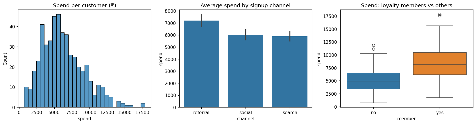
Step 8: Conclusions#
Write findings as short statements backed by numbers from the analysis above, and note what the data cannot tell you:
- A typical customer places a handful of orders a year and spends a few thousand rupees; spend is right-skewed, so the median is a better "typical" value than the mean.
- Referral customers spend the most on average, ahead of search and social, though they are the smallest channel. Referral programmes may be worth expanding.
- Loyalty members order more often and spend substantially more, and the difference is far too large to be chance (very small p-value).
- Caveat: this is observational data. Members may spend more because keen customers join the programme, not because the programme makes them spend. An experiment (offering membership to a random group) would be needed to measure its effect.
Practice#
Practice exercise
Extend the analysis: using customers_clean.csv, compute the average spend per order (spend ÷ orders, for customers with at least one order) for each city, sorted from highest to lowest. Does any city stand out?
Show hint
Filter orders > 0, add a per_order column, then groupby("city")["per_order"].mean().
Show solution
import pandas as pd

df = pd.read_csv("customers_clean.csv")
active = df[df["orders"] > 0].copy()
active["per_order"] = active["spend"] / active["orders"]
print(active.groupby("city")["per_order"].mean().round(0).sort_values(ascending=False))city
Delhi 994.0
Mumbai 990.0
Chennai 971.0
Pune 968.0
Bengaluru 962.0
Name: per_order, dtype: float64The averages are close across cities, so no city stands out on value per order; differences in total spend come mainly from how many customers and orders each city has.
Key takeaway#
Next project: Monthly Sales Report.
Finished this lesson?