Python for Data course menu
Choosing the Right Chart: Bar, Line, Scatter, Histogram and Box Plot
Pick the right chart for your data with matplotlib examples: bar charts for comparisons, line charts for trends, scatter plots for relationships, histograms and box plots for distributions, and why pie charts are usually a poor choice.
On this page
The right chart makes the answer obvious; the wrong one hides it. Start from the question, then pick the chart:
Bar charts: comparing categories#
import matplotlib.pyplot as plt

cities = ["Mumbai", "Delhi", "Bengaluru", "Pune", "Chennai"]
orders = [480, 420, 390, 210, 180]

fig, ax = plt.subplots(figsize=(7, 4))
bars = ax.barh(cities[::-1], orders[::-1], color="#4C72B0")
ax.bar_label(bars, padding=3)
ax.set_title("Orders by city")
ax.set_xlabel("Orders")
plt.tight_layout()
plt.show()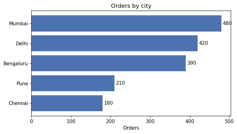
- Horizontal bars (
barh) leave room for long category names. - Sort the bars so the ranking is obvious.
- Bars must start at zero: bar length represents the value.
bar_labelwrites the values on the bars, so readers do not have to estimate.
Grouped bars#
import numpy as np
import matplotlib.pyplot as plt

quarters = ["Q1", "Q2", "Q3", "Q4"]
year_2025 = [120, 135, 150, 170]
year_2026 = [140, 150, 165, 195]
x = np.arange(len(quarters))
width = 0.38

fig, ax = plt.subplots(figsize=(7, 4))
ax.bar(x - width / 2, year_2025, width, label="2025", color="#A1A9B3")
ax.bar(x + width / 2, year_2026, width, label="2026", color="#4C72B0")
ax.set_xticks(x, quarters)
ax.set_title("Revenue by quarter")
ax.set_ylabel("Revenue (₹ lakh)")
ax.legend()
plt.show()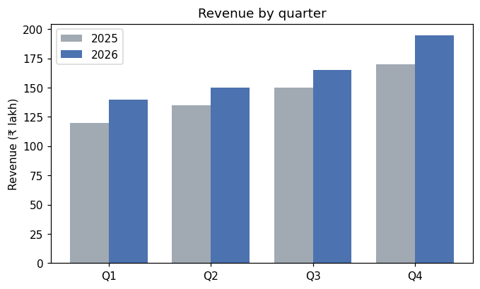
Using grey for the older year and a strong colour for the current one draws attention where it belongs.
Line charts: trends over time#
Use lines when the x axis is time (or another ordered quantity). See matplotlib Basics for examples. Avoid lines between unordered categories: a line from "Mumbai" to "Delhi" means nothing.
Scatter plots: relationships#
import numpy as np
import matplotlib.pyplot as plt

rng = np.random.default_rng(4)
ad_spend = rng.uniform(10, 100, 50)
sales = 3 * ad_spend + rng.normal(0, 25, 50)

fig, ax = plt.subplots(figsize=(6, 4))
ax.scatter(ad_spend, sales, alpha=0.7)
slope, intercept = np.polyfit(ad_spend, sales, 1)
xs = np.array([10, 100])
ax.plot(xs, slope * xs + intercept, color="#C44E52", label=f"trend: {slope:.2f} per ₹1k")
ax.set(xlabel="Ad spend (₹ thousands)", ylabel="Sales (units)", title="Ad spend vs sales")
ax.legend()
plt.show()
print(round(slope, 2), round(intercept, 1))3.08 -5.5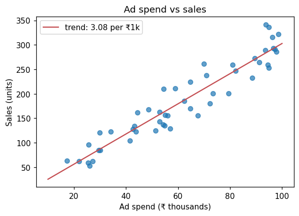
np.polyfit(x, y, 1) fits a straight line; the slope says how many extra units sell per extra ₹1,000 of advertising in this simulated data. Use alpha (transparency) when points overlap.
Histograms and box plots: distributions#
import numpy as np
import matplotlib.pyplot as plt

rng = np.random.default_rng(8)
teams = {
    "Team A": rng.normal(30, 5, 200),
    "Team B": rng.normal(35, 9, 200),
    "Team C": rng.exponential(8, 200) + 22,
}

fig, axes = plt.subplots(1, 2, figsize=(11, 4))
axes[0].hist(teams["Team A"], bins=25, color="#4C72B0", edgecolor="white")
axes[0].set(title="Team A resolution times", xlabel="Minutes", ylabel="Tickets")
axes[1].boxplot(list(teams.values()), tick_labels=list(teams.keys()))
axes[1].set(title="All teams", ylabel="Minutes")
plt.tight_layout()
plt.show()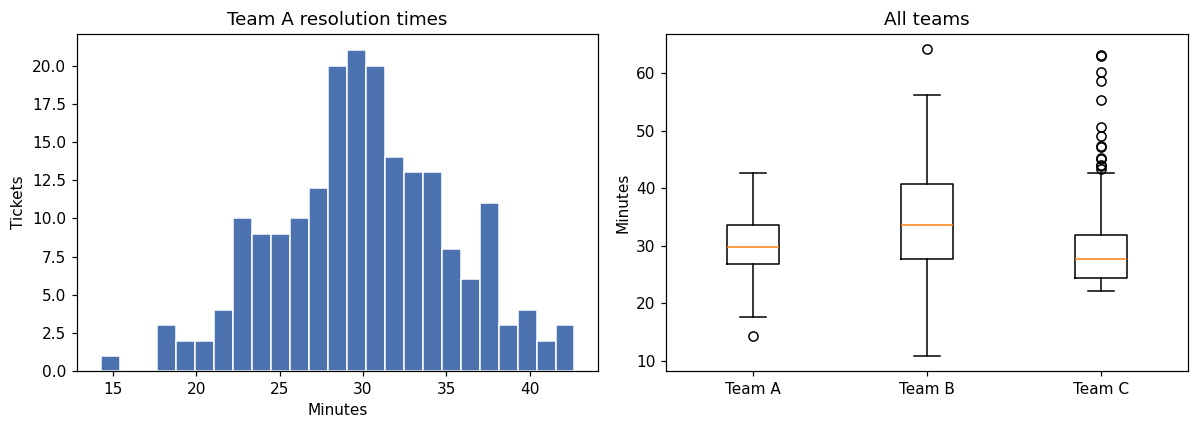
A box plot shows the median (line), the middle 50% of values (the box, from Q1 to Q3), the whiskers (up to 1.5 × IQR) and outliers (dots). It is the best way to compare distributions across groups side by side.
What about pie charts?#
People compare lengths far more accurately than angles. With more than two or three slices, or slices of similar size, a sorted bar chart is easier to read than a pie. If you need "share of the total", a single stacked or 100% bar usually works better.
Common mistakes#
Practice#
Practice exercise
Survey answers to "How satisfied are you?" were: Very satisfied 42, Satisfied 85, Neutral 30, Unsatisfied 12, Very unsatisfied 6. Draw a horizontal bar chart in the natural order of the answers (not sorted by size), with value labels, and print the percentage who were satisfied or very satisfied.
Show hint
Ordered categories (like a rating scale) should keep their natural order. barh draws the first item at the bottom, so reverse the lists to put "Very satisfied" on top.
Show solution
import matplotlib.pyplot as plt

answers = ["Very satisfied", "Satisfied", "Neutral", "Unsatisfied", "Very unsatisfied"]
counts = [42, 85, 30, 12, 6]

fig, ax = plt.subplots(figsize=(7, 3.5))
bars = ax.barh(answers[::-1], counts[::-1], color="#55A868")
ax.bar_label(bars, padding=3)
ax.set(title="Customer satisfaction", xlabel="Responses")
plt.tight_layout()
plt.show()
print(f"{(42 + 85) / sum(counts):.1%}")72.6%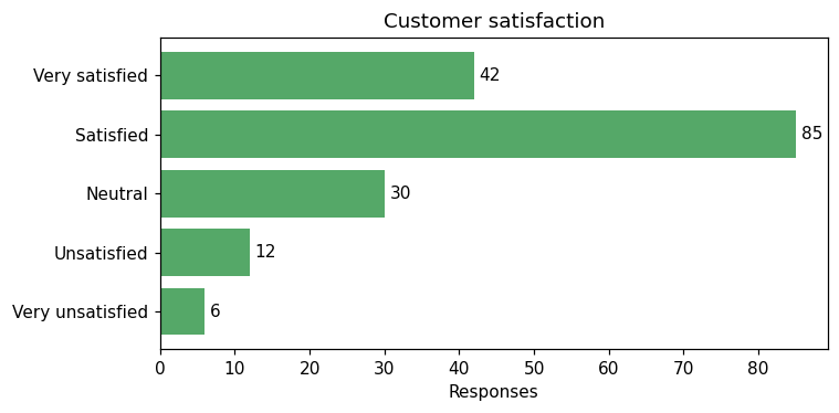
Key takeaway#
Next: Subplots, Labels and Styling.
Finished this lesson?