Data Distributions in Python: Histograms, Normal Distribution and Z-scores

A distribution describes how often each value occurs: which values are common, which are rare, and whether the data is symmetric or lopsided. Two datasets can have the same mean and standard deviation but very different shapes, so it pays to look.

Histograms show the shape#

A histogram splits the range of values into bins and counts how many values fall into each. Here are 1,000 simulated heights (normally distributed) and 1,000 simulated delivery times (right-skewed):

import numpy as np
import matplotlib.pyplot as plt

rng = np.random.default_rng(7)
heights = rng.normal(loc=165, scale=8, size=1000)
deliveries = rng.exponential(scale=10, size=1000) + 20

fig, axes = plt.subplots(1, 2, figsize=(10, 4))
axes[0].hist(heights, bins=30, color="#4C72B0", edgecolor="white")
axes[0].set_title("Heights (cm): symmetric")
axes[1].hist(deliveries, bins=30, color="#DD8452", edgecolor="white")
axes[1].set_title("Delivery time (min): right-skewed")
for ax in axes:
    ax.set_ylabel("Count")
plt.tight_layout()
plt.show()

print(round(heights.mean(), 1), round(np.median(heights), 1))
print(round(deliveries.mean(), 1), round(np.median(deliveries), 1))

164.4 164.5
30.2 26.9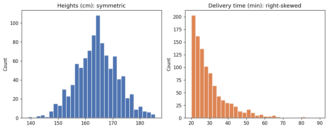

For the symmetric heights, mean and median are almost equal. For the skewed delivery times, the long right tail pulls the mean above the median.

The normal distribution#

The normal (Gaussian) distribution is the familiar bell curve. It is described by its mean μ (the centre) and standard deviation σ (the width). Many measurements are roughly normal: heights, measurement errors, averages of many small effects.

The 68-95-99.7 rule: about 68% of values lie within 1σ of the mean, 95% within 2σ and 99.7% within 3σ. We can check it on simulated data:

import numpy as np

rng = np.random.default_rng(7)
heights = rng.normal(loc=165, scale=8, size=100_000)
for k in [1, 2, 3]:
    within = (np.abs(heights - 165) <= k * 8).mean()
    print(f"within {k} sd: {within:.1%}")

within 1 sd: 68.3%
within 2 sd: 95.4%
within 3 sd: 99.8%

Exact probabilities with scipy.stats#

scipy.stats.norm gives exact normal probabilities. cdf(x) is the probability of a value at most x; ppf(p) goes the other way and gives the value below which a fraction p falls:

from scipy.stats import norm

mu, sigma = 165, 8
print(round(norm.cdf(173, mu, sigma), 4))                          # P(height <= 173)
print(round(1 - norm.cdf(181, mu, sigma), 4))                      # P(height > 181)
print(round(norm.cdf(173, mu, sigma) - norm.cdf(157, mu, sigma), 4))  # within 1 sd
print(round(norm.ppf(0.95, mu, sigma), 1))                         # 95th percentile

0.8413
0.0228
0.6827
178.2

Exactly 68.27% lies within one standard deviation, which is where the "68" in the rule comes from. A height of 181 cm (2σ above the mean) is exceeded by only about 2.3% of people.

Z-scores#

A z-score expresses a value as "how many standard deviations from the mean": z = (x − μ) / σ. It puts values on different scales on a common footing:

import pandas as pd

scores = pd.DataFrame({
    "subject": ["Maths", "English"],
    "score": [78, 82],
    "class_mean": [65, 78],
    "class_std": [10, 4],
})
scores["z"] = (scores["score"] - scores["class_mean"]) / scores["class_std"]
print(scores)

   subject  score  class_mean  class_std    z
0    Maths     78          65         10  1.3
1  English     82          78          4  1.0

82 in English looks better than 78 in Maths, but relative to their classes, the Maths score is stronger (1.3 standard deviations above the mean versus 1.0).

Other common shapes#

Skewed data is often analysed on a log scale (np.log), which makes it closer to symmetric.

Common mistakes#

Practice#

from scipy.stats import norm

print(round(1 - norm.cdf(90, 70, 12), 3))
print(round(norm.cdf(80, 70, 12) - norm.cdf(60, 70, 12), 3))
print(round(norm.ppf(0.9, 70, 12), 1))

0.048
0.595
85.4

Key takeaway#

Next: how two variables move together, in Correlation.